
Jolt is a RISC-V zkVM uniquely designed around sumcheck and lookup arguments (Just One Lookup Table).
Jolt is fast (state-of-the-art performance on CPU) and relatively simple (thanks to its lookup-centric architecture).
AI coding agents: Install the Jolt agent skill to let Claude Code, Cursor, Codex, etc. wrap Rust functions in Jolt proofs: npx skills add a16z/jolt
This book has the following top-level sections:
- Intro (you are here)
- Usage (how to use Jolt in your applications)
- How it works (how the proof system and implementation work under the hood)
- Roadmap (what's next for Jolt)
Related reading
Papers
Jolt: SNARKs for Virtual Machines via Lookups
Arasu Arun, Srinath Setty, Justin Thaler
Twist and Shout: Faster memory checking arguments via one-hot addressing and increments
Srinath Setty, Justin Thaler
Unlocking the lookup singularity with Lasso
Srinath Setty, Justin Thaler, Riad Wahby
Blog posts
Initial launch:
Updates:
- Nov 12, 2024 blog video
- Aug 18, 2025 (Twist and Shout upgrade) blog
- Oct 15, 2025 (RV64 support) blog
Background
Credits
Jolt was initially forked from Srinath Setty's work on microsoft/Spartan, specifically the arkworks-rs/Spartan fork in order to use the excellent arkworks-rs field and curve implementations.
Jolt uses its own fork of arkworks-algebra with certain optimizations, including some described here.
Jolt's R1CS is also proven using a version of Spartan (forked from the microsoft/Spartan2 codebase) optimized for Jolt's uniform R1CS constraints.
Jolt uses Dory as its PCS, inspired by the Space and Time Labs implementation spaceandtimefdn/sxt-dory.
Usage
Quickstart
AI Coding Skill
Install the Jolt agent skill to let AI coding agents (Claude Code, Cursor, Codex, etc.) wrap Rust functions in Jolt proofs for you:
npx skills add a16z/jolt
Fallback (Claude Code / Codex):
curl -sfL jolt.rs/skill | bash
Installing
Start by installing the jolt command line tool.
cargo install --git https://github.com/a16z/jolt --force --bins jolt
Creating a Project
To create a project, use the jolt new command.
jolt new <PROJECT_NAME>
This will create a template Jolt project in the specified location. Make sure to cd into the project before running the next step.
cd <PROJECT_NAME>
Project Tour
The main folder contains the host, which is the code that can generate and verify proofs. Within this main folder, there is another package called guest which contains the Rust functions that we can prove from the host. For more information about these concepts refer to the guests and hosts section.
We'll start by taking a look at our guest. We can view the guest code in guest/src/lib.rs.
#![allow(unused)]
#![cfg_attr(feature = "guest", no_std)]

fn main() {
#[jolt::provable(heap_size = 32768, max_trace_length = 65536)]
fn fib(n: u32) -> u128 {
    let mut a: u128 = 0;
    let mut b: u128 = 1;
    let mut sum: u128;
    for _ in 1..n {
        sum = a + b;
        a = b;
        b = sum;
    }

    b
}
}
As we can see, this implements a simple Fibonacci function called fib. All we need to do to make our function provable is add the jolt::provable macro above it. The generated guest/src/main.rs contains the #![no_main] binary stub that lets Jolt build a RISC-V ELF, while guest/src/lib.rs contains the provable functions you edit.
Next let's take a look at the host code in src/main.rs.
use tracing::info;

pub fn main() {
    tracing_subscriber::fmt::init();

    let target_dir = "/tmp/jolt-guest-targets";
    let mut program = guest::compile_fib(target_dir);

    let shared_preprocessing = guest::preprocess_shared_fib(&mut program).unwrap();

    let prover_preprocessing = guest::preprocess_prover_fib(shared_preprocessing.clone());
    let verifier_setup = prover_preprocessing.generators.to_verifier_setup();
    let verifier_preprocessing =
        guest::preprocess_verifier_fib(shared_preprocessing, verifier_setup, None);

    let prove_fib = guest::build_prover_fib(program, prover_preprocessing);
    let verify_fib = guest::build_verifier_fib(verifier_preprocessing);

    let (output, proof, io_device) = prove_fib(50);
    let is_valid = verify_fib(50, output, io_device.panic, proof);

    info!("output: {output}");
    info!("valid: {is_valid}");
}
The host uses functions generated by the jolt::provable macro. The pipeline has four stages:
- Compile —
compile_fibcompiles the guest to RISC-V. - Preprocess —
preprocess_shared_fibproduces shared preprocessing, which is then split into prover and verifier preprocessing. This only depends on the program (not inputs) and can be reused across proofs. The last argument topreprocess_verifier_fibisNonefor ordinary proofs; ZK proofs passSome(blindfold_setup)instead. - Prove —
build_prover_fibreturns a closure with the same inputs as the original function. It returns the output, a proof, and anio_device(which includes apanicflag). - Verify —
build_verifier_fibreturns a closure that takes the public inputs, claimed output, panic flag, and proof, returning a boolean.
Running
Let's now run the host with cargo.
cargo run --release
This will compile the guest, perform preprocessing, and execute the host code which proves and verifies the 50th Fibonacci number. Preprocessing only needs to be performed once for a given program, and can be reused to prove multiple invocations.
Note that many logs in the example are logged at the info level. To see these logs, you can set the RUST_LOG environment variable before running the host:
RUST_LOG=info cargo run --release
If everything is working correctly, you should see output similar to the following:
...
2025-11-05T22:17:43.849979Z  INFO jolt_prover_legacy::zkvm: Proved in 2.6s (0.4 kHz / padded 0.8 kHz)
2025-11-05T22:17:43.923164Z  INFO example: output: 12586269025
2025-11-05T22:17:43.923300Z  INFO example: valid: true
Development
Rust
To build Jolt from source, you will need Rust:
curl --proto '=https' --tlsv1.2 -sSf https://sh.rustup.rs | sh- Rustup should automatically install the Rust toolchain and necessary targets on
the first
cargoinvocation. You may also need to add the RISC-V target for building guest programs manually:rustup target add riscv64imac-unknown-none-elf.
mdBook
To build this book from source:
cargo install mdbook mdbook-katex
For watching the changes in your local browser:
mdbook watch book --open
Guests and Hosts
Guests and hosts are the main concepts that we need to understand in order to use Jolt as an application developer. Guests contain the functions that Jolt will prove, while hosts are where we invoke the prover and verifier for our guest functions.
Guests
Guests contain functions for Jolt to prove. Making a function provable is as easy as ensuring it is inside the guest package and adding the jolt::provable macro above it.
Let's take a look at a simple guest program to better understand it.
#![allow(unused)]
#![cfg_attr(feature = "guest", no_std)]

fn main() {
#[jolt::provable]
fn add(x: u32, y: u32) -> u32 {
    x + y
}
}
As we can see, the guest looks like a normal no_std Rust library. The only major change is the addition of the jolt::provable macro, which lets Jolt know of the function's existence. The only requirement of these functions is that its inputs are serializable and outputs are deserializable with serde. Fortunately serde is prevalent throughout the Rust ecosystem, so most types will support it by default.
There is no requirement that just a single function lives within the guest, and we are free to add as many as we need. Additionally, we can import any no_std compatible library just as we normally would in Rust.
#![allow(unused)]
#![cfg_attr(feature = "guest", no_std)]

fn main() {
use sha2::{Sha256, Digest};
use sha3::{Keccak256, Digest};

#[jolt::provable]
fn sha2(input: &[u8]) -> [u8; 32] {
    let mut hasher = Sha256::new();
    hasher.update(input);
    let result = hasher.finalize();
    Into::<[u8; 32]>::into(result)
}

#[jolt::provable]
fn sha3(input: &[u8]) -> [u8; 32] {
    let mut hasher = Keccak256::new();
    hasher.update(input);
    let result = hasher.finalize();
    Into::<[u8; 32]>::into(result)
}
}
Prover and Verifier Views of Guest Program
A guest program consists of two main components: program code and inputs. Both the prover and verifier know the program code (and how it compiles to RISC-V instructions).
Jolt supports three types of inputs:
-
Public Input: These are inputs known to both the prover and verifier. The prover proves that given the bytecode and these inputs, the claimed output is correct.
-
Untrusted Advice (
jolt::UntrustedAdvice<T>): These inputs are known to the prover for generating the proof, but the verifier does not receive them. The prover proves that there exists some input that produces the claimed output. Note:UntrustedAdvicedoes not guarantee privacy — without thezkfeature, polynomial evaluations are revealed in the clear and the inputs may be extractable from the proof. -
Private Input (
jolt::PrivateInput<T>): Equivalent toUntrustedAdvice<T>but signals that the input should be cryptographically hidden from the verifier via the BlindFold protocol. Thezkfeature must be enabled onjolt-sdkin the host crate; the guest needs no feature flag. The#[jolt::provable]macro enforces this at compile time. -
Trusted Advice (
jolt::TrustedAdvice<T>): Similar to untrusted advice, but the verifier has a commitment to the input generated by an external party (not the prover). The prover proves that there exists an input matching the given commitment that, when executed with the program code, produces the claimed output.
A program can use any combination of these input types. To access the inner value, dereference the wrapper with *.
Private inputs (ZK)
When you need inputs that are cryptographically hidden from the verifier, use PrivateInput<T>. Enable the zk feature on jolt-sdk in the host crate — the guest needs no feature flag. You can scaffold a ZK-ready project with jolt new my-project --zk.
Guest Cargo.toml (no zk feature needed):
[dependencies]
jolt = { package = "jolt-sdk" }
Host Cargo.toml:
[dependencies]
jolt-sdk = { features = ["host", "zk"] }
If the guest uses PrivateInput<T> but the host doesn't enable zk, compilation fails with a clear error message.
Guest (guest/src/lib.rs):
#![allow(unused)]
#![cfg_attr(feature = "guest", no_std)]
fn main() {
use jolt::PrivateInput;

#[jolt::provable(heap_size = 32768, max_trace_length = 65536)]
fn fib(n: PrivateInput<u32>) -> u128 {
    let mut a: u128 = 0;
    let mut b: u128 = 1;
    for _ in 1..*n {
        let sum = a + b;
        a = b;
        b = sum;
    }
    b
}
}
Host (src/main.rs):
#![allow(unused)]
fn main() {
use jolt_sdk::PrivateInput;

let verifier_setup = prover_preprocessing.generators.to_verifier_setup();
let blindfold_setup = prover_preprocessing.blindfold_setup();
let verifier_preprocessing =
    guest::preprocess_verifier_fib(shared_preprocessing, verifier_setup, Some(blindfold_setup));

// Prover receives the private input
let (output, proof, io_device) = prove_fib(PrivateInput::new(50));

// Verifier does not — it only sees the output and proof
let is_valid = verify_fib(output, io_device.panic, proof);
}
The generated verifier closure omits private and advice parameters — only public inputs appear in the verifier's signature.
For a complete example of advice inputs, see the merkle-tree example.
Zero knowledge
By default, the prover reveals polynomial evaluations in the clear. To produce zero-knowledge proofs where the verifier learns nothing beyond the validity of the output, enable the zk feature on jolt-sdk in the host crate. This activates the BlindFold protocol, which commits all sumcheck round polynomials via Pedersen and proves correctness via Nova folding + Spartan.
PrivateInput<T> is always available in the guest. If you use UntrustedAdvice<T> without zk, the verifier won't receive the inputs, but the proof itself does not hide them cryptographically.
The generated preprocess_verifier_* function always takes three arguments: shared, generators, and Option<BlindfoldSetup<Bn254Curve>>. Pass Some(blindfold_setup) when using zk mode, or None otherwise.
Advice inputs vs. runtime advice
Advice inputs described above (UntrustedAdvice<T>, PrivateInput<T>, TrustedAdvice<T>) are host-provided: the host supplies the data before execution, and it is written into a preallocated memory region that the guest reads from. The guest program runs once, and the values are fixed before execution begins.
Runtime advice is a separate mechanism where the guest itself computes advice values during a first-pass execution, and those values are fed back via an advice tape for the proving pass. This is useful when the advice depends on the guest's own execution (e.g. computing a modular inverse or finding factors) and checking the result is cheaper than computing it. Runtime advice uses #[jolt::advice] functions rather than wrapper-type parameters on #[jolt::provable].
Both mechanisms signal that the data is untrusted and must be verified by the guest, but they differ in where the data originates and how it is serialized (advice inputs use serde; runtime advice uses AdviceTapeIO).
Security model
Beyond the usual Rust rules around unsafe and undefined behavior, Jolt guest programs are subject to a few zkVM-specific rules:
-
Self-modifying programs are undefined behavior. Jolt commits to the program's bytecode at preprocessing time. A guest that writes to its own code region can still produce a valid proof, but the semantics of that proof are undefined — the proof attests to execution against the committed bytecode, not the modified version.
-
Direct invocation of Jolt's custom RISC-V instructions is unsafe. Jolt extends the RISC-V ISA with custom instructions used internally (e.g. for inline cryptographic primitives and runtime advice). Invoking these instructions directly from guest code, such as via inline assembly, bypasses the safety checks performed by the SDK and may produce incorrect proofs or cause proving to fail.
-
Prover-supplied advice must be validated by the guest.
UntrustedAdvice<T>andPrivateInput<T>are supplied by the prover and are not constrained by the proof system itself. The guest is responsible for verifying that any advice it consumes satisfies the properties the program relies on (e.g. that a claimed factor actually divides the input, or that a claimed Merkle path matches a known root).TrustedAdvice<T>carries an external commitment, but the data itself may still require validation. -
No source of randomness or wall clock. The guest has no entropy source and no clock. The platform exposes
sys_rand(seejolt-platform/src/random.rs), but it is a deterministic PRNG seeded with a fixed constant — its output is fully predictable, including by the verifier — and is not suitable for cryptographic use. Any value that must be unpredictable (nonces, keys, sampling weights) has to be supplied as a public input. Supplying it via advice does not solve the problem: advice is chosen by the prover, so a "key" derived from advice is a key the prover picked. -
Bytecode is public. The compiled guest ELF is committed at preprocessing time and is known to the verifier. The
zkfeature protects inputs, not the program. Do not embed secrets in guest code — API keys, hardcoded credentials, or proprietary algorithms you do not want disclosed. -
Outputs and the panic flag are public. The return value and
io_device.panicare revealed to the verifier and are what the proof attests to. Returning a value derived from a private input leaks that value; panicking conditionally on a private input leaks one bit per panic site. Guests handling secret data should be written so that the output and panic behavior depend only on public information. -
Output byte representation. The output memory region is zero-initialized, and both prover and verifier strip trailing zero bytes before binding outputs to the Fiat-Shamir transcript. As a result, byte strings that differ only in trailing zeros (e.g.,
[0x41]vs[0x41, 0x00]) produce identical proofs. Typed outputs are unaffected — the SDK restores the full serialized length before deserialization — but protocols that consumeprogram_io.outputsas raw bytes must not treat trailing zeros as semantically meaningful, or must encode an explicit length. -
No side-channel resistance. The
zkfeature, via the BlindFold protocol, makes proofs zero-knowledge with respect to the verifier. However, Jolt's prover implementation is not constant-time and makes no claims of resistance to side-channel attacks. A party that observes prover execution (timing, memory access patterns, power consumption, etc.) may learn information about private inputs. Do not run the prover on secret data in adversarial environments without additional mitigations.
Standard Library
Jolt supports the Rust standard library. To enable support, simply add the guest-std feature to the Jolt import in the guest's Cargo.toml file and remove the #![cfg_attr(feature = "guest", no_std)] directive from the guest code.
Example
#![allow(unused)]
fn main() {
[package]
name = "guest"
version = "0.1.0"
edition = "2021"

[features]
guest = []

[dependencies]
jolt = { package = "jolt-sdk", git = "https://github.com/a16z/jolt", features = ["guest-std"] }
}
#![allow(unused)]

fn main() {
#[jolt::provable]
fn int_to_string(n: i32) -> String {
    n.to_string()
}
}
alloc
Jolt provides an allocator which supports most containers such as Vec and Box. This is useful for Jolt users who would like to write no_std code rather than using Jolt's standard library support. To use these containers, they must be explicitly imported from alloc. The alloc crate is automatically provided by rust and does not need to be added to the Cargo.toml file.
Example
#![allow(unused)]
#![cfg_attr(feature = "guest", no_std)]

fn main() {
extern crate alloc;
use alloc::vec::Vec;

#[jolt::provable]
fn alloc(n: u32) -> u32 {
    let mut v = Vec::<u32>::new();
    for i in 0..100 {
        v.push(i);
    }

    v[n as usize]
}
}
Print statements
Jolt supports standard print! and println! macros in guest programs.
Example
#![allow(unused)]
fn main() {
#[jolt::provable(heap_size = 10240, max_trace_length = 65536)]
fn int_to_string(n: i32) -> String {
    print!("Hello, ");
    println!("from int_to_string({n})!");
    n.to_string()
}
}
The printed strings are written to stdout during RISC-V emulation of the guest.
Optimization level
By default, the guest program is compiled with optimization level 3 to attempt to minimize the number of RISC-V instructions executed during emulation.
To change this optimization level, set the JOLT_GUEST_OPT environment variable to one of the allowed values: 0, 1, 2, 3, s, or z.
A common choice is z which optimizes for code size, at the cost of a larger number of instructions executed.
Hosts
Hosts are where we can invoke the Jolt prover to prove functions defined within the guest.
The host imports the guest package, and will have automatically generated functions to build each of the Jolt functions. For the SHA3 example we looked at in the guest section, the jolt::provable procedural macro generates several functions that can be invoked from the host (shown below):
compile_sha3(target_dir)compiles the SHA3 guest to RISC-V.preprocess_shared_sha3(&mut program)produces shared preprocessing from the compiled program. This only needs to be generated once and can be reused across proofs.preprocess_prover_sha3(shared)andpreprocess_verifier_sha3(shared, verifier_setup, blindfold_setup)produce prover and verifier preprocessing from the shared preprocessing. The verifier setup is obtained fromprover_pp.generators.to_verifier_setup(). PassNonefor ordinary proofs, orSome(prover_pp.blindfold_setup())when proving with thezkfeature.build_prover_sha3returns a closure for the prover, which takes in the same input types as the original function and returns the output, a proof, and aprogram_iodevice.build_verifier_sha3returns a closure for the verifier. The verifier closure's parameters comprise of the program input, the claimed output, aboolvalue claiming whether the guest panicked, and the proof.
use std::time::Instant;

pub fn main() {
    let target_dir = "/tmp/jolt-guest-targets";
    let mut program = guest::compile_sha3(target_dir);

    let shared_preprocessing = guest::preprocess_shared_sha3(&mut program).unwrap();
    let prover_preprocessing = guest::preprocess_prover_sha3(shared_preprocessing.clone());
    let verifier_setup = prover_preprocessing.generators.to_verifier_setup();
    let verifier_preprocessing =
        guest::preprocess_verifier_sha3(shared_preprocessing, verifier_setup, None);

    let prove_sha3 = guest::build_prover_sha3(program, prover_preprocessing);
    let verify_sha3 = guest::build_verifier_sha3(verifier_preprocessing);

    let input: &[u8] = &[5u8; 32];
    let now = Instant::now();
    let (output, proof, program_io) = prove_sha3(input);
    println!("Prover runtime: {} s", now.elapsed().as_secs_f64());
    let is_valid = verify_sha3(input, output, program_io.panic, proof);

    println!("output: {}", hex::encode(output));
    println!("valid: {is_valid}");
}
Memory management
To reduce peak memory usage during proving, replace the default system allocator with jemalloc. The default system allocator retains freed pages in the process's address space for reuse, which inflates RSS beyond actual live memory. jemalloc returns freed pages to the OS more aggressively via madvise, keeping RSS close to true usage at a modest proving time cost.
# your-host/Cargo.toml
[dependencies]
tikv-jemallocator = "0.6"
#![allow(unused)]
fn main() {
// your-host/src/main.rs
#[global_allocator]
static GLOBAL: tikv_jemallocator::Jemalloc = tikv_jemallocator::Jemalloc;
}
#[global_allocator] must be declared in your final binary crate — Jolt SDK is a library and cannot set it for you.
This is most useful in containers, on shared machines where RSS determines whether you get OOM-killed, or for client-side proving where the prover runs on consumer hardware with limited memory. If you have plenty of memory and want the fastest possible proving, stick with the default allocator.
Runtime Advice
Runtime advice allows guest programs to offload expensive computations to the prover and receive the results via an advice tape. The guest then verifies the result cheaply, rather than recomputing it from scratch. This can dramatically reduce cycle counts for operations like modular inversion, factoring, or any computation where checking a result is cheaper than computing it.
Runtime advice is distinct from the advice inputs (TrustedAdvice<T> / UntrustedAdvice<T> parameters on #[jolt::provable]), which are host-provided data fixed before execution begins. With runtime advice, the guest itself computes the values during a first-pass execution, and those values are replayed from the advice tape during the proving pass. Use advice inputs when the host already knows the auxiliary data; use runtime advice when the data depends on the guest's own logic and checking is cheaper than computing.
How it works
Jolt uses a two-pass execution model for advice:
- First pass (compute_advice): The guest is compiled with the
compute_advicefeature flag. Advice functions execute their body and write results to the advice tape. - Second pass (proving): The guest is compiled without
compute_advice. Advice functions read precomputed results from the advice tape instead of recomputing them.
The prover handles both passes automatically. The guest code only needs to define advice functions and verify their outputs.
Defining advice functions
Annotate a function with #[jolt::advice]. The function must return jolt::UntrustedAdvice<T>, where T implements AdviceTapeIO.
#![allow(unused)]
fn main() {
use jolt::AdviceTapeIO;

#[jolt::advice]
fn modinv_advice(a: u64, m: u64) -> jolt::UntrustedAdvice<(u64, u64)> {
    // This body only runs during the compute_advice pass.
    // During proving, the result is read from the advice tape.
    let inv = extended_gcd(a, m);
    let quo = (a as u128 * inv as u128 / m as u128) as u64;
    (inv, quo)
}
}
Requirements:
- The return type must be
jolt::UntrustedAdvice<T> - Arguments must be immutable (no
mutor&mut) Tmust implementAdviceTapeIO(see Supported types below)
Verifying advice
Advice values are untrusted -- the prover could supply arbitrary data. The guest must verify correctness using check_advice! or check_advice_eq!. These macros emit prover-enforced assertions: if the condition is false, proof generation fails.
#![allow(unused)]
fn main() {
#[jolt::provable]
fn modinv(a: u64, m: u64) -> u64 {
    let adv = modinv_advice(a, m);
    let (inv, quo) = *adv;  // Deref to access the inner value

    // Verify: a * inv ≡ 1 (mod m)
    let product = (a as u128) * (inv as u128) - (quo as u128) * (m as u128);
    jolt::check_advice!(product == 1u128 && inv < m);

    inv
}
}
check_advice_eq! is a specialization for equality checks that directly compares two register-sized values, saving a few instructions compared to check_advice!:
#![allow(unused)]
fn main() {
jolt::check_advice_eq!(a * b, n, "incorrect factors");
jolt::check_advice!(1 < a && a <= b && b < n, "factors out of range");
}
Both macros accept an optional error message string as the last argument. The message is used in assert!/assert_eq! on non-RISC-V targets (useful for debugging) but is stripped from the guest binary.
Supported types
The AdviceTapeIO trait controls how values are serialized to and from the advice tape. Built-in implementations are provided for:
| Type | Notes |
|---|---|
u8, u16, u32, u64, usize | Primitive integers |
i8, i16, i32, i64 | Signed integers |
[T; N] where T: Pod | Fixed-size arrays |
(A, B), ..., (A, B, C, D, E, F, G) | Tuples up to 7 elements |
Vec<T> where T: Pod | Requires guest-std feature |
Custom structs
For structs composed of supported types, you can implement AdviceTapeIO manually:
#![allow(unused)]
fn main() {
struct Pair {
    x: u64,
    y: u64,
}

impl jolt::AdviceTapeIO for Pair {
    fn write_to_advice_tape(&self) {
        self.x.write_to_advice_tape();
        self.y.write_to_advice_tape();
    }
    fn new_from_advice_tape() -> Self {
        Pair {
            x: u64::new_from_advice_tape(),
            y: u64::new_from_advice_tape(),
        }
    }
}
}
JoltPod: automatic AdviceTapeIO via bytemuck
For #[repr(C)] structs where all fields are plain-old-data, you can derive AdviceTapeIO automatically using bytemuck and the JoltPod marker trait:
#![allow(unused)]
fn main() {
use bytemuck_derive::{Pod, Zeroable};
use jolt::JoltPod;

#[derive(Copy, Clone, Pod, Zeroable)]
#[repr(C)]
struct Point {
    x: u32,
    y: u32,
}
impl JoltPod for Point {}
}
JoltPod types get a blanket AdviceTapeIO implementation that uses bytemuck for zero-copy serialization. This works for nested structs too, as long as all types in the hierarchy are Pod.
Guest setup
The guest Cargo.toml must include a compute_advice feature:
[package]
name = "guest"
version = "0.1.0"
edition = "2021"

[features]
guest = []
compute_advice = []

[dependencies]
jolt = { package = "jolt-sdk", git = "https://github.com/a16z/jolt" }
The compute_advice feature is used by the SDK to build the first-pass binary. You do not need to activate it yourself.
Full example
Guest (guest/src/lib.rs):
#![allow(unused)]
fn main() {
use jolt::AdviceTapeIO;

/// Compute factors of n via advice (expensive trial division runs outside the proof)
#[jolt::advice]
fn factor(n: u32) -> jolt::UntrustedAdvice<[u32; 2]> {
    for i in 2..=n {
        if n % i == 0 {
            return [i, n / i];
        }
    }
    [1, n]
}

/// Prove that n is composite by obtaining and verifying its factors via advice
#[jolt::provable]
fn verify_composite(n: u32) {
    let adv = factor(n);
    let [a, b] = *adv;

    // Verify the factors are correct and non-trivial
    jolt::check_advice_eq!((a as u64) * (b as u64), n as u64);
    jolt::check_advice!(1 < a && a <= b && b < n);
}
}
Host (src/main.rs):
pub fn main() {
    let target_dir = "/tmp/jolt-guest-targets";

    let mut program = guest::compile_verify_composite(target_dir);
    let shared_preprocessing = guest::preprocess_shared_verify_composite(&mut program);
    let prover_preprocessing =
        guest::preprocess_prover_verify_composite(shared_preprocessing.clone());
    let verifier_setup = prover_preprocessing.generators.to_verifier_setup();
    let verifier_preprocessing =
        guest::preprocess_verifier_verify_composite(shared_preprocessing, verifier_setup);

    let prove = guest::build_prover_verify_composite(program, prover_preprocessing);
    let verify = guest::build_verifier_verify_composite(verifier_preprocessing);

    let n = 221u32;  // 13 * 17
    let (output, proof, program_io) = prove(n);
    let is_valid = verify(n, output, program_io.panic, proof);
    assert!(is_valid);
}
The host code is identical to any other Jolt program. The two-pass advice mechanism is handled transparently by the compile_* and build_prover_* functions generated by the #[jolt::provable] macro.
Profiling
If you're an application developer, you may want to profile your guest program: fewer cycles = faster proof. If so, check out Guest profiling.
If you're contributing to Jolt, you may be interested in profiling Jolt itself, in which case you should check out zkVM profiling
Profiling Jolt
Execution profiling
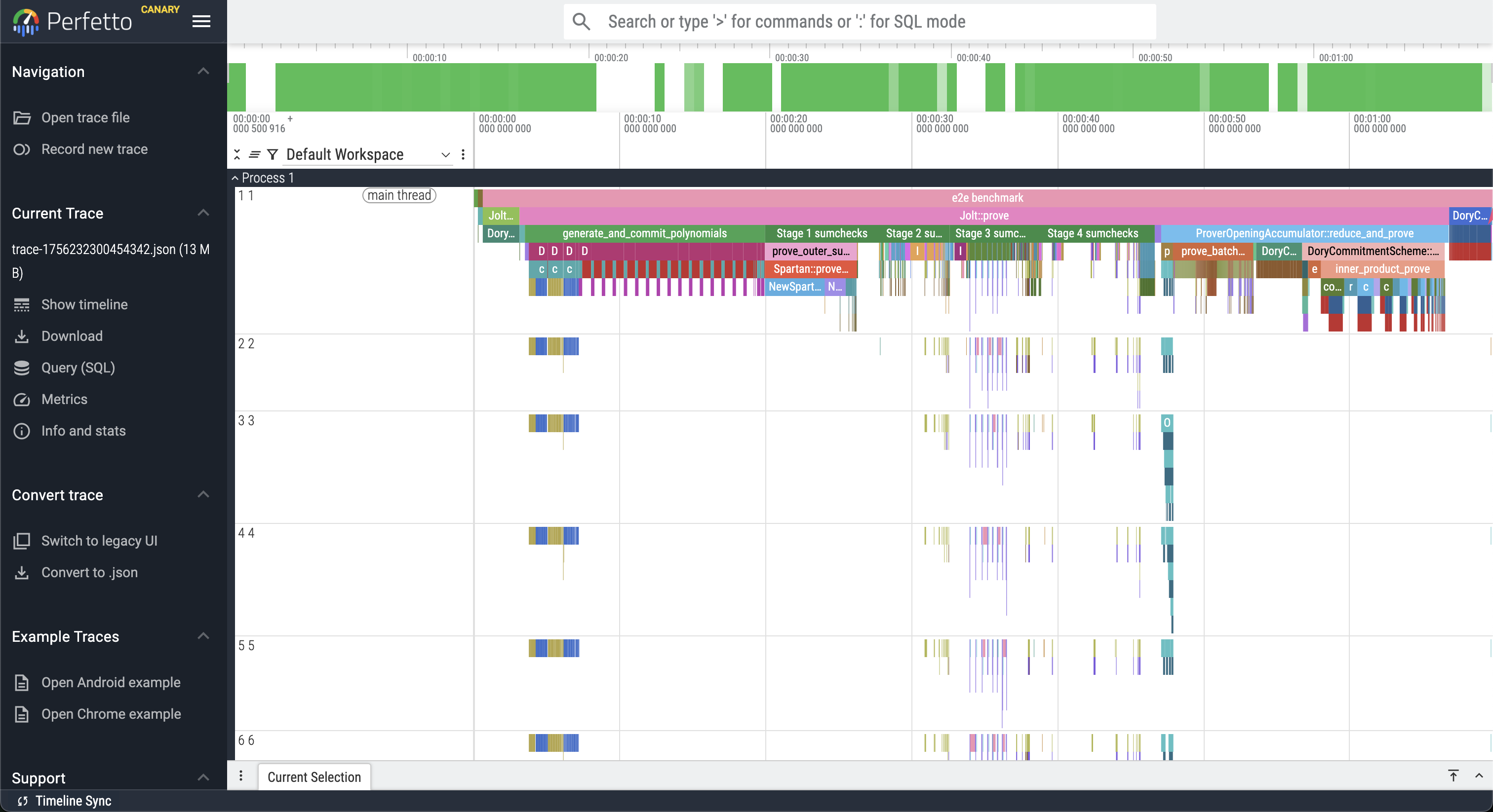
Jolt is instrumented using tokio-rs/tracing for execution profiling.
We use the tracing_chrome crate to output traces in the format expected by Perfetto.
To generate a trace, run e.g.
cargo run --release -p jolt-prover-legacy profile --name sha3 --format chrome
Where --name can be sha2, sha3, sha2-chain, fibonacci, or btreemap. The corresponding guest programs can be found in the examples directory. The benchmark inputs are provided in bench.rs.
The above command will output a JSON file in the workspace rootwith a name trace-<timestamp>.json, which can be viewed in Perfetto:
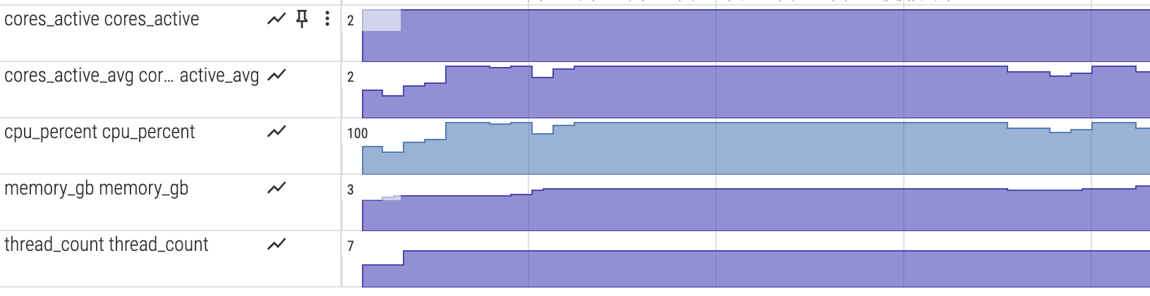
System resource monitoring
To visualize CPU and memory usage alongside the execution trace, enable the monitor feature:
cargo run --release --features monitor -p jolt-prover-legacy profile --name sha3 --format chrome
python3 scripts/postprocess_trace.py trace-*.json
The postprocessing step converts the metrics into counter tracks for Perfetto.
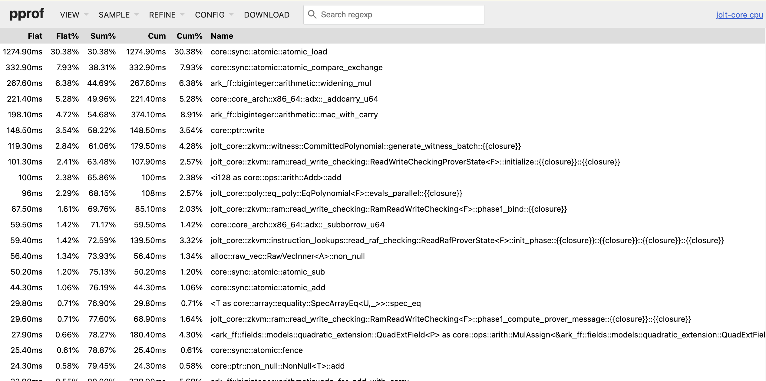
Fine-grained CPU profiling with pprof
When tracing is insufficiently detailed, you can enable pprof for fine-grained CPU profiling. While execution tracing shows you the high-level stages and their durations (based on manually instrumented code), pprof automatically samples your entire program at the function level to capture each function call including in dependencies. This can help reveal performance bottlenecks that tracing might miss, such as unexpected hotspots in serialization, memory allocation, or cryptographic operations.
To enable pprof profiling, add the --features pprof flag:
cargo run --release --features pprof -p jolt-prover-legacy profile --name sha3 --format chrome
This will generate multiple .pb profile files in benchmark-runs/pprof/, one for each major stage.
To view the proving profile in your browser using pprof, run:
go tool pprof -http=:8080 target/release/jolt-prover-legacy benchmark-runs/pprof/sha3_prove.pb
This will start a web server at http://localhost:8080 where you can explore:
- Flame graphs - Visual representation of call stacks and time spent
- Top functions - List of functions consuming the most CPU time
- Source view - Line-by-line breakdown of CPU usage
- Call graph - Function call relationships
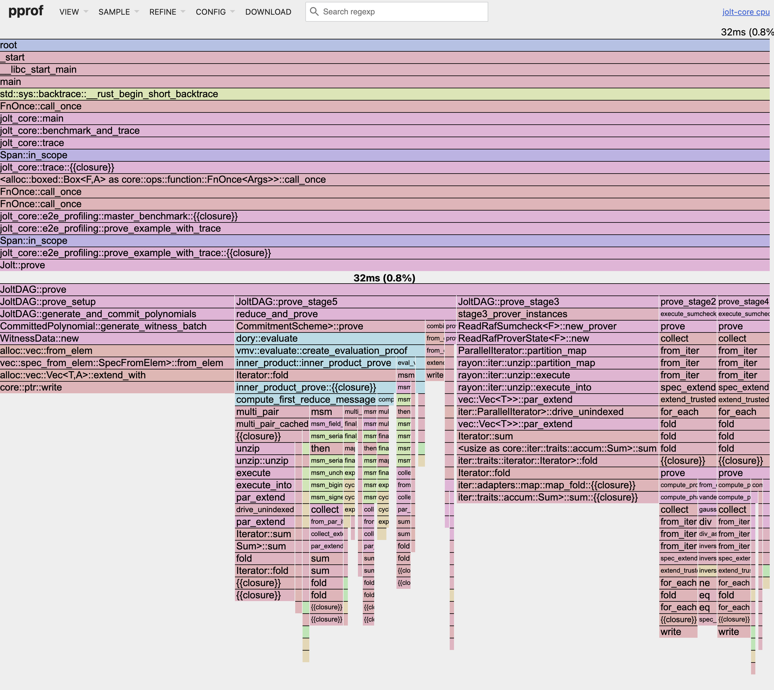
You may need to increase the sampling frequency to get a more detailed profile for shorter traces or decrease it for longer tracesto reduce overhead.You may customize the sampling frequency using the PPROF_FREQ environment variable (default: 100 Hz):
PPROF_FREQ=1000 cargo run --release --features pprof -p jolt-prover-legacy profile --name sha3 --format chrome
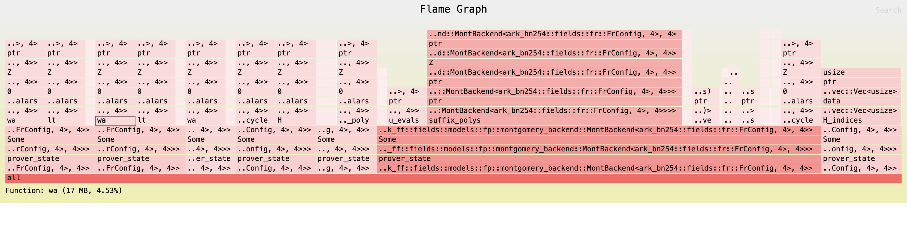
Memory profiling
Jolt uses allocative for memory profiling.
Allocative allows you to (recursively) measure the total heap space occupied by any data structure implementing the Allocative trait, and optionally generate a flamegraph.
In Jolt, most sumcheck data structures implement the Allocative trait, and we generate a flamegraph at the start and end of stages 2-7 (see crates/jolt-prover-legacy/src/zkvm/prover.rs).
To generate allocative output, run:
RUST_LOG=debug cargo run --release --features allocative -p jolt-prover-legacy profile --name sha3 --format chrome
Where, as above, --name can be sha2, sha3, sha2-chain, fibonacci, or btreemap.
The above command will log memory usage info to the command line and output multiple SVG files, e.g. stage3_start_flamechart.svg, which can be viewed in a web browser of your choosing:
Guest Profiling
This section details the available tools to profile guest programs. There is currently a single utility available: Cycle-Tracking, which is detailed below.
Cycle-Tracking in Jolt
Measure real (RV64IMAC) and virtual cycles inside your RISC-V guest code with zero-overhead markers. This is useful when analyzing the mapping between the high-level guest program and the equivalent compiled program to be proven by Jolt.
Note: The Rust compiler will often shuffle around your implementation for optimization purposes, which can affect cycle tracking. If you suspect the compiler is interfering with profiling, then use the Hint module. For example, wrap values in
core::hint::black_box()(see below) to help keep your measurements honest.
API
| Function | Effect |
|---|---|
start_cycle_tracking(label: &str) | Begin a span tagged with label |
end_cycle_tracking(label: &str) | End the span started with the same label |
Under the hood each marker emits an ECALL signaling the emulator to track your code segment.
Example
#![allow(unused)]
#![cfg_attr(feature = "guest", no_std)]
fn main() {
use jolt::{start_cycle_tracking, end_cycle_tracking};

#[jolt::provable]
fn fib(n: u32) -> u128 {
    let (mut a, mut b) = (0, 1);

    start_cycle_tracking("fib_loop");
    for _ in 1..n {
        let sum = a + b;
        a = b;
        b = sum;
    }
    end_cycle_tracking("fib_loop");

    b
}
}
Hinting the compiler
#![allow(unused)]
#![cfg_attr(feature = "guest", no_std)]
fn main() {
use core::hint::black_box;

#[jolt::provable]
fn muldiv(a: u32, b: u32, c: u32) -> u32 {
    use jolt::{end_cycle_tracking, start_cycle_tracking};

   start_cycle_tracking("muldiv");
   let result = black_box(a * b / c); // use black_box to keep code in place
   end_cycle_tracking("muldiv");

   result
}
}
Wrap inputs or outputs that must stay observable during the span. In the above example, a * b / c gets moved to the return line without black_box(), causing inaccurate measurements. To run the above example, use cargo run --release -p muldiv.
Expected Output
"muldiv": 9 RV64IMAC cycles, 16 virtual cycles
Trace length: 533
Prover runtime: 0.487551667 s
output: 2223173
valid: true
Troubleshooting
Insufficient Memory or Stack Size
Jolt provides reasonable defaults for the total allocated memory and stack size. It is however possible that the defaults are not sufficient, leading to unpredictable errors within our tracer. To fix this we can try to increase these sizes. We suggest starting with the stack size first as this is much more likely to run out.
Below is an example of manually specifying both the total memory and stack size.
#![allow(unused)]
#![cfg_attr(feature = "guest", no_std)]
#![no_main]

fn main() {
extern crate alloc;
use alloc::vec::Vec;

#[jolt::provable(stack_size = 10000, heap_size = 10000000)]
fn waste_memory(size: u32, n: u32) {
    let mut v = Vec::new();
    for i in 0..size {
        v.push(i);
    }
}
}
Maximum Input or Output Size Exceeded
Jolt restricts the size of the inputs and outputs to 4096 bytes by default. Using inputs and outputs that exceed this size will lead to errors. These values can be configured via the macro.
#![allow(unused)]
#![cfg_attr(feature = "guest", no_std)]
#![no_main]

fn main() {
#[jolt::provable(max_input_size = 10000, max_output_size = 10000)]
fn sum(input: &[u8]) -> u32 {
    let mut sum = 0;
    for value in input {
        sum += *value as u32;
    }

    sum
}
}
Guest Attempts to Compile Standard Library
Sometimes after installing the toolchain the guest still tries to compile with the standard library which will fail with a large number of errors that certain items such as Result are referenced and not available. This generally happens when one tries to run jolt before installing the toolchain. To address, try rerunning jolt install-toolchain, restarting your terminal, and delete both your rust target directory and any files under /tmp that begin with jolt.
Guest Fails to Compile on the Host
By default, Jolt will attempt to compile the guest for the host architecture. This is useful if you want to run and test the guest's tagged functions directly. If you know your guest code cannot compile on the host (for example, if your guest uses inline RISCV assembly), you can specify to only build for the guest architecture.
#![allow(unused)]
fn main() {
#[jolt::provable(guest_only)]
fn inline_asm() -> (i32, u32, i32, u32) {
    use core::arch::asm;

    let mut data: [u8; 8] = [0; 8];
    unsafe {
        let ptr = data.as_mut_ptr();

        // Store Byte (SB instruction)
        asm!(
        "sb {value}, 0({ptr})",
        ptr = in(reg) ptr,
        value = in(reg) 0x12,
        );
    }
}
}
Null Pointer Write / "Unknown memory mapping: 0x0"
If you see Null pointer write detected (store to 0x0) or Illegal device store: Unknown memory mapping: 0x0, it means your guest program crashed. This happens when musl's abort() cannot deliver a signal and falls back to writing to a null pointer.
The most common cause is a missing jolt-sdk feature. If your guest uses:
- rayon or threading — add
"thread"to your jolt-sdk features - randomness (getrandom) — add
"random"to your jolt-sdk features
[dependencies]
jolt = { package = "jolt-sdk", features = ["guest-std", "thread", "random"] }
To diagnose which syscall is failing, add the "debug" feature to enable syscall logging:
jolt = { package = "jolt-sdk", features = ["guest-std", "debug"] }
This prints every syscall the guest makes (e.g. [syscall] SYS_clone), which helps identify which capability is missing.
Release runs with fat LTO fail a lookup-table test
If cargo nextest run --release -p jolt-prover-legacy fails at:
'zkvm::lookup_table::equal::test::prefix_suffix' panicked at crates/jolt-prover-legacy/src/zkvm/lookup_table/test.rs:108:17:
assertion `left == right` failed
this appears to be a fat LTO miscompile in the current compiler pass pipeline. This class of miscompilations is generally tracked in rust-lang/rust#116941.
Workarounds
- Prefer thin LTO (default in
Cargo.toml):profile.release.lto = "thin"
- If you must keep fat LTO, disable LLVM prepopulate passes (use Cargo’s profile override
to avoid applying LTO to proc-macro/build scripts):
CARGO_PROFILE_RELEASE_LTO=fat RUSTFLAGS="-C no-prepopulate-passes"
These avoid the miscompile while keeping release runs functional.
LTO Configuration Details
We have investigated three primary LTO configurations.
1. lto = "fat" (Problematic)
Enabling "fat" LTO without additional flags triggers a compiler miscompilation in the current toolchain.
To reproduce:
CARGO_PROFILE_RELEASE_LTO=fat cargo nextest run --release -p jolt-prover-legacy -E 'test(=zkvm::lookup_table::equal::test::prefix_suffix)'
You will see an error similar to:
thread 'zkvm::lookup_table::equal::test::prefix_suffix' panicked at crates/jolt-prover-legacy/src/zkvm/lookup_table/test.rs:108:17:
assertion `left == right` failed
  left: 3421757210433941145757981284077922153733430471292915370254709621273756639318
 right: 15993602859885613318374216934674599210221976492830069114166327961258944178919
2. lto = "thin" (Recommended)
The above error can be fixed by setting lto = "thin". You can verify with:
CARGO_PROFILE_RELEASE_LTO=thin cargo nextest run --release -p jolt-prover-legacy -E 'test(=zkvm::lookup_table::equal::test::prefix_suffix)'
3. lto = "fat" with -C no-prepopulate-passes
If you must use fat LTO, adding RUSTFLAGS="-C no-prepopulate-passes" prevents the miscompilation described above. However, this flag alters the guest ELF code generation, which can increase the execution trace length slightly.
This may cause tests with tight trace length limits—such as advice_e2e_dory—to fail.
To reproduce:
CARGO_PROFILE_RELEASE_LTO=fat RUSTFLAGS="-C no-prepopulate-passes" cargo nextest run --release -p jolt-prover-legacy -E 'test(=zkvm::prover::tests::advice_e2e_dory)'
You will see a trace length error:
    thread 'zkvm::prover::tests::advice_e2e_dory' panicked at crates/jolt-prover-legacy/src/zkvm/prover.rs:336:13:
    Execution trace length (105501 cycles, padded to 131072) exceeds max_trace_length (65536) configured in MemoryConfig. Increase max_trace_length to at least 131072.
To fix this, simply increase the max_trace_length in the failing test setup. For example, in advice_e2e_dory:
let shared_preprocessing = JoltSharedPreprocessing::new(
    bytecode.clone(),
    io_device.memory_layout.clone(),
    init_memory_state,
-   1 << 16,
+   1 << 17,
);
Getting Help
If none of the above solve the problem, please create a Github issue with a detailed bug report including the Jolt commit hash, the hardware or container configuration used, and a minimal guest program to reproduce the bug.
How it works
This section dives into in the inner workings of Jolt, beyond what an application developer needs to know. It covers the architecture, design decisions, and implementation details of Jolt. Proceed if you:
-
have been poking around the Jolt codebase and have questions about why something is implemented the way it is
-
have read some papers (Jolt, Twist/Shout) and want to know how things fit together in practice
-
would like to start contributing to Jolt
This section is comprised of the following subsections:
Architecture overview
This section gives a overview of the architecture of the Jolt codebase.
The following diagram depicts the end-to-end Jolt pipeline, which is typical of RISC-V zkVMs.
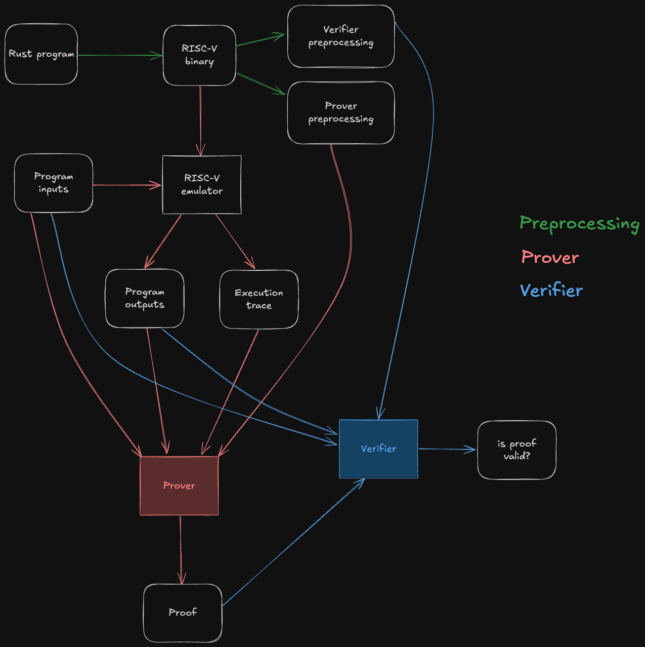
The green steps correspond to preprocessing steps, which can be computed ahead of time from the guest program's bytecode. Note that they do not depend on the program inputs, so the preprocessing data can be reused across multiple invocations of the Jolt prover/verifier.
The red steps correspond to the prover's workflow: it runs the guest program on some inputs inside of a RISC-V emulator, producing the output of the program as well as an execution trace. This execution trace, along with the inputs, outputs, and preprocessing, are then passed to the Jolt prover, which uses them to generate a succinct proof that the outputs are the result of correctly executing the given guest program on the inputs.
The blue steps correspond to the verifier's workflow. The verifier does not emulate the guest program, not does it receive the execution trace (which may be billions of cycles long) from the prover. Instead, it receives the proof from the prover, and uses it to check that the guest program produces claimed outputs when run on the given inputs.
For the sake of readability, the diagram above abstracts away all of Jolt's proof system machinery. The rest of this section aims to disassemble the underlying machinery in useful-but-not-overwhelming detail.
As a starting point, we will present two useful mental models of the Jolt proof system: Jolt as a CPU, and Jolt as a DAG (a different DAG than the one above; we love DAGs).
Jolt as a CPU
One way to understand Jolt is to map the components of the proof system to the components of the virtual machine (VM) whose functionality they prove.
Jolt's five components
A VM does two things:
- Repeatedly execute the fetch-decode-execute logic of its instruction set architecture.
- Perform reads and writes to memory.
The Jolt paper depicts these two tasks mapped to three components in the Jolt proof system:
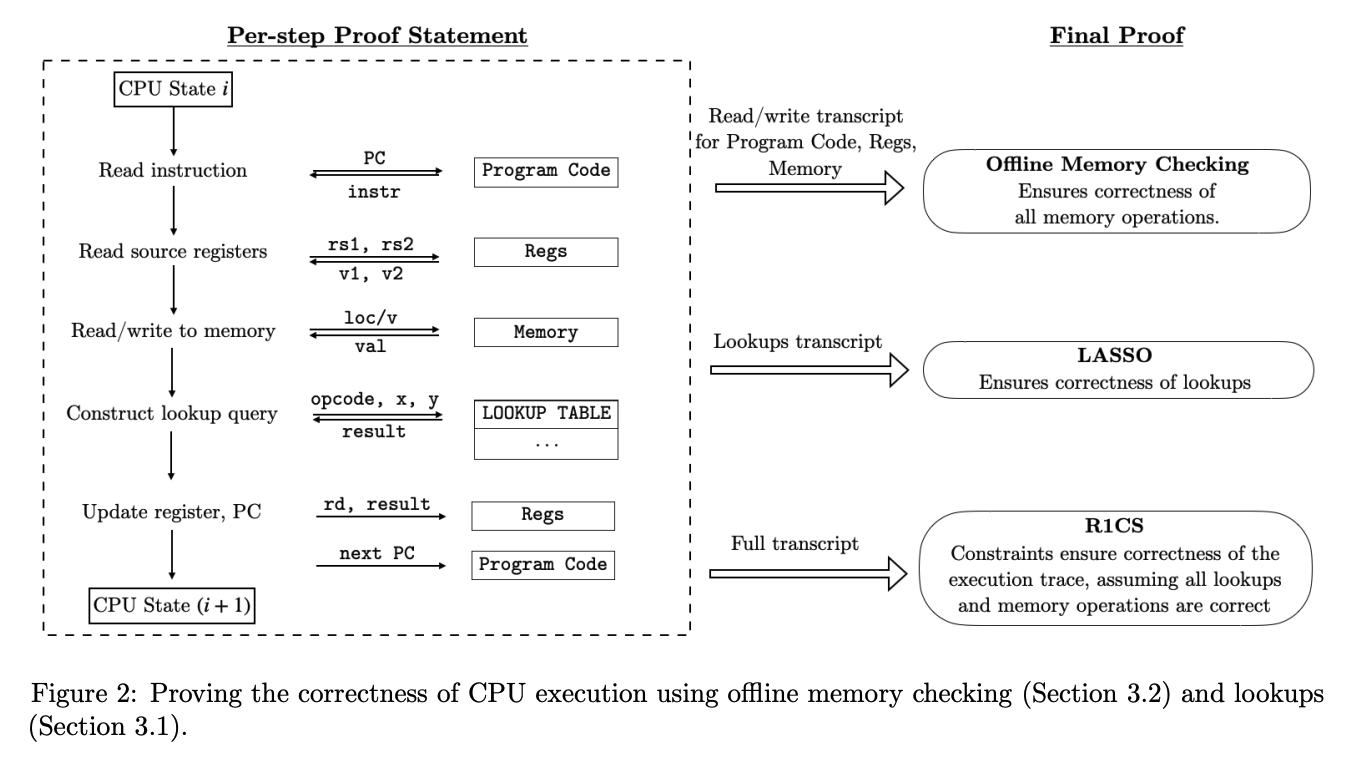
The Jolt codebase is similarly organized, but instead distinguishes read-write memory (comprising registers and RAM) from program code (aka bytecode, which is read-only), for a total of five components:
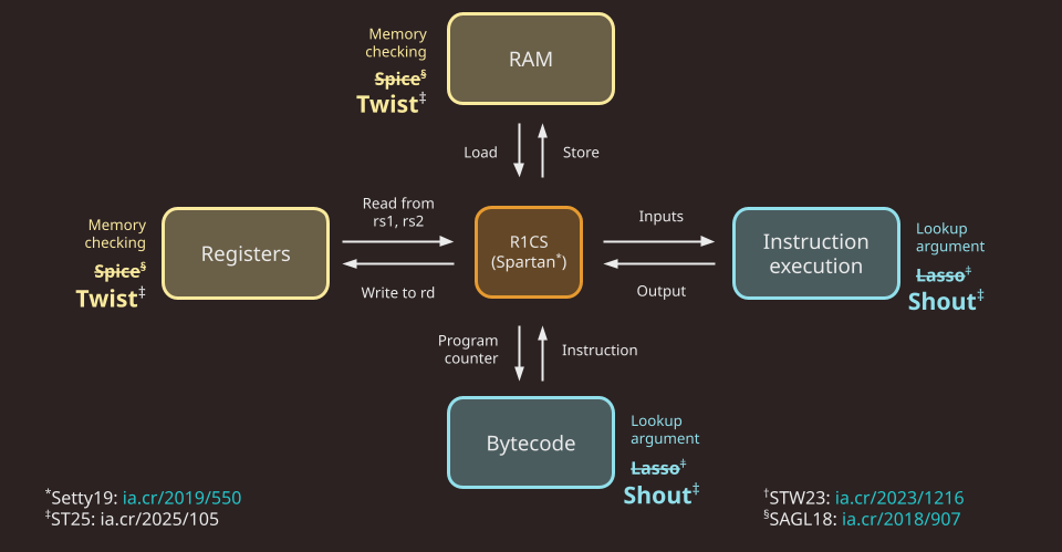
Note that in Jolt as described in the paper, as well as in the first version of the Jolt implementation (v0.1.0), the memory checking and lookup argument used are Spice and Lasso, respectively. As of v0.2.0, Jolt replaces Spice and Lasso with Twist and Shout, respectively.
R1CS constraints
To handle the "fetch" part of the fetch-decode-execute loop, there is a minimal R1CS instance (about 20 constraints per cycle of the RISC-V VM). These constraints handle program counter (PC) updates and serves as the "glue" enforcing consistency between polynomials used in the components below. Jolt uses Spartan, optimized for the highly-structured nature of the constraint system (i.e. the same small set of constraints are applied to every cycle in the execution trace).
For more details: R1CS constraints
RAM
To handle reads/writes to RAM Jolt uses the Twist memory checking argument.
For more details: RAM
Registers
Similar to RAM, Jolt uses the Twist memory checking argument to handle reads/writes to registers.
For more details: Registers
Instruction execution
To handle the "execute" part of the fetch-decode-execute loop, Jolt invokes the Shout lookup argument. The lookup table, in this case, effectively maps every instruction to its correct output.
For more details: Instruction execution
Bytecode
To handle the "decode" part of the fetch-decode-execute loop, Jolt uses another instance of Shout. The bytecode of the guest program is "decoded" in preprocessing, and the prover subsequently invokes offline memory-checking on the sequence of reads from this decoded bytecode corresponding to the execution trace being proven.
For more details: Bytecode
Jolt as a DAG
One useful way to understand Jolt is to view it as a directed acyclic graph (DAG). That might sound surprising -- how can a zkVM be represented as a DAG? The key lies in the structure of its sumchecks, and in particular, the role of virtual polynomials.
Virtual vs. Committed Polynomials
Virtual polynomials, a concept introduced in the Binius paper, are used heavily in Jolt.
A virtual polynomial is a part of the witness that is never committed directly. Instead, any claimed evaluation of a virtual polynomial is proven by a subsequent sumcheck. In contrast, committed polynomials are committed to explicitly and their evaluaions are proven using the opening proof of the PCS.
Sumchecks as Nodes
Each sumcheck in Jolt corresponds to a node in the DAG. Consider the following hypothetical sumcheck expression:
Here, the left-hand side is the input claim, and the right-hand side is a sum over the Boolean hypercube of a multivariate polynomial of degree 2, involving three multilinear terms , , and . The sumcheck protocol reduces this input claim to three output claims about , , and :
where consists of the random challenges obtained over the course of the sumcheck.
An output claim of one sumcheck might be the input claim of another sumcheck. Recall that by definition, the output claim for a virtual polynomial is necessarily the input claim of another sumcheck.
It follows that input claims can be viewed as in-edges and output claims as out-edges, thus defining the graph structure. This is what the Jolt sumcheck DAG looks like:
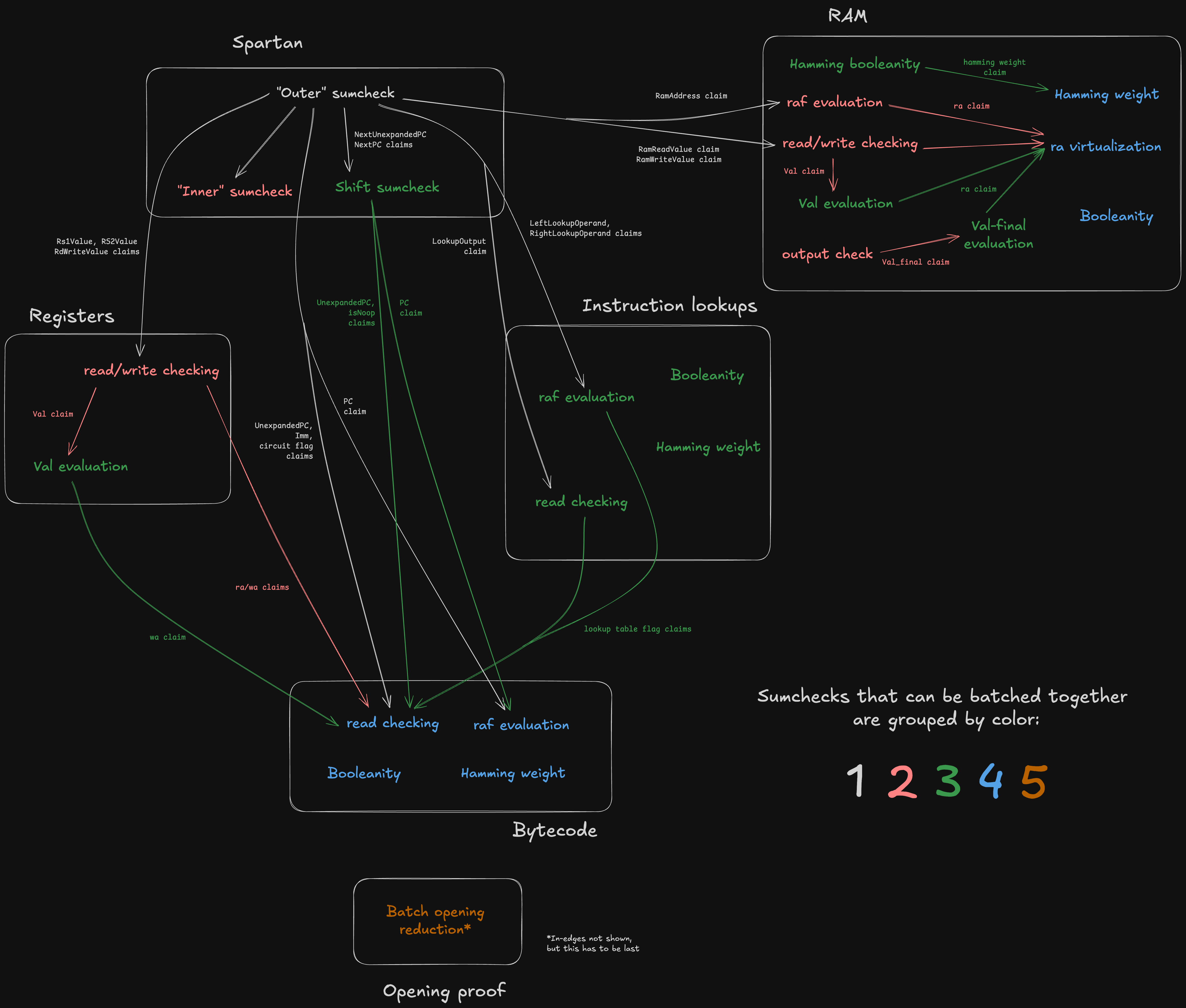
Note the white boxes corresponding to the five components of Jolt under the CPU paradigm –– plus two extra components ("R1CS input virtualization" and "One-hot checks") which don't have a CPU analogue.
In the diagaram above, sumchecks are color-coded based on "batch"; sumchecks in the same batch are "run in parallel" (see Batched sumcheck). Note that a given component may include sumchecks in different batches. For example, the sumchecks under "Registers" span stages 3, 4, 5, and 6.
The sumcheck stages are codified in zkvm/prover.rs (resp. zkvm/verifier.rs), which contain functions prove_stage1, prove_stage2 (resp. verify_stage1, verify_stage2) etc.
The function for a given stage declares which sumcheck instances the stage contains.
Observe that the DAG defines a partial ordering over the nodes (sumchecks), which consequently defines the minimum number of batches -- two sumchecks cannot be batched together if one "depends" on the other.
The terminal nodes in the graph –– namely, the "Inc claim reduction" and the Hamming weight + ra claim reduction" –– output claims that are directly proven using the PCS opening proof. For more details on the batched opening proof subprotocol, see Opening proof.
Managing state and data flow
The ProverOpeningAccumulator (resp. VerifierOpeningAccumulator) is responsible for managing the flow of opening claims –– the edges of the DAG.
The opening accumulator contains a mapping from OpeningId to claimed polynomial evaluation.
As sumchecks are proven, their output claims (for both virtual and committed polynomials) are inserted into the map. Later sumchecks can then consume the virtual polynomial openings as input claims.
While virtual polynomial claims are used internally and passed between sumchecks, committed polynomial claims are tracked because they must ultimately be verified via a batched Dory opening proof at the end of the protocol.
The input_claim and cache_openings methods on the SumcheckInstanceProver and SumcheckInstanceVerifier traits provide hooks to the respective accumulator objects.
input_claim effectively declares the in-edges for the sumcheck instance, while cache_openings effectively declares the out-edges.
RISC-V emulation
Jolt's RISC-V emulator is implemented within the tracer crate.
It originated as a fork of the riscv-rust project and has since evolved significantly to support Jolt’s unique requirements.
The bulk of the emulator's logic resides in the instruction subdirectory of the tracer crate, which defines the behavior of individual RISC-V instructions.
Privilege and Trap Model
Jolt's RISC-V implementation targets M-mode-only execution with no interrupt hardware. All guest programs run under ZeroOS, a minimal runtime that operates exclusively in Machine mode. There are no S-mode or U-mode privilege levels, no timer, no CLINT, no PLIC, and no external interrupt sources.
This model has the following consequences for privileged instructions:
-
ECALL writes
mepc,mcause,mtval, andmstatusto their virtual registers, then jumps tomtvec.mstatusis set to0x1800(MPP = M-mode, MIE = 0, MPIE = 0) unconditionally rather than via read-modify-write. This is correct because the privilege mode is always M-mode, and interrupt-enable bits are unused — the MIE CSR (0x304) is not in the supported CSR whitelist and cannot be accessed by guest code. -
MRET jumps to
mepcand does not modifymstatus. The full RISC-V spec requires restoringMIEfromMPIEand resettingMPP, but these fields are inert in the M-mode-only model. The ZeroOS trap trampoline restoresmstatusviacsrwbefore executingmret, so the virtual register always holds the correct value. -
CSR access is restricted to a fixed whitelist:
mstatus(0x300),mtvec(0x305),mscratch(0x340),mepc(0x341),mcause(0x342),mtval(0x343). Accessing any other CSR panics the tracer. OnlyCSRRWandCSRRSare implemented;CSRRCand the immediate CSR variants are not supported. -
The R1CS constraint system has no privilege-mode or interrupt semantics. CSR virtual registers (vr34–vr39) are treated as ordinary registers by the memory-checking circuit. The circuit verifies read/write consistency, not the architectural meaning of individual bits.
Core traits
Two key traits form the backbone of the RISC-V emulator:
-
RISCVInstruction- Defines core instruction behavior required by the tracer.
- Includes two associated constants,
MASKandMATCH, used for decoding instructions from raw bytes. - Has an associated type
Format, indicating the RISC-V instruction format (e.g., R-type or I-type). - The associated type
RAMAccessspecifies memory access (read/write) required by the instruction, guiding the tracer in capturing memory state before and after execution. - Its critical method,
execute, emulates instruction execution by modifying CPU state and populating memory state changes as needed.
-
RISCVTrace(extendsRISCVInstruction)- Adds a
tracemethod, which by default invokesexecuteand additionally captures pre- and post-execution states of any accessed registers or memory. May be overridden for instructions which employ virtual sequences, see below. - Constructs a
RISCVCyclestruct instance from the captured information and appends it to a trace vector.
- Adds a
Core enums
Instruction and Cycle are enums encapsulating all RV64IMAC instruction variants, wrapping implementations of RISCVInstruction and RISCVCycle, respectively.
Virtual Instructions and Sequences
A crucial concept in Jolt is that of virtual instructions and virtual sequences, introduced in section 6 of the Jolt paper. Virtual instructions don't exist in the official RISC-V ISA but are specifically created to facilitate proving.
Reasons for Using Virtual Instructions:
Complex operations (e.g. division)
Some instructions, like division, don't neatly adhere to the lookup table structure required by prefix-suffix Shout. To handle these cases, the problematic instruction is expanded into a virtual sequence, a series of instructions (some potentially virtual).
For instance, division involves a sequence described in detail in section 6.3 of the Jolt paper, utilizing virtual untrusted "advice" instructions. In the context of division, the advice instructions store the quotient and remainder in virtual registers, which are additional registers used exclusively within virtual sequences as scratch space. The rest of the division sequence verifies the correctness of the computed quotient and remainder, finally storing the quotient in the destination register specified by the original instruction.
Atomic operations (LR/SC)
The RISC-V "A" extension's Load-Reserved/Store-Conditional (LR/SC) instructions are implemented using virtual sequences with dedicated reservation registers. These are a pair of width-specific virtual registers that track the address reserved by the most recent LR instruction:
reservation_w(virtual register 32): Set byLR.W, checked bySC.Wreservation_d(virtual register 33): Set byLR.D, checked bySC.D
When LR.W executes, it writes the reservation address into reservation_w (vr32) and clears reservation_d (vr33). Conversely, LR.D writes into reservation_d (vr33) and clears reservation_w (vr32). This cross-clear mechanism prevents mixed-width LR/SC pairing: an SC.W after LR.D will always fail because the word-width reservation register was cleared by the LR.D.
SC failure path
SC.W and SC.D must handle both success and failure within the zkVM's constraint system. This is accomplished using VirtualAdvice:
- The prover supplies a success/failure bit via
VirtualAdvice, constrained to usingVirtualAssertLTE. - A derived
v_successflag () gates the reservation check: . On success (), this forces the reservation to match the target address. On failure (), the constraint is trivially satisfied. - The store is conditional: . On success this writes
rs2; on failure it writes back the original memory value (a no-op). - The destination register is set to 0 on success, 1 on failure.
Soundness: A malicious prover cannot claim success without a valid reservation, because the constraint would be violated. However, the prover can claim spurious failure even with a valid reservation, which is permitted by the RISC-V specification (SC is allowed to fail spuriously).
Per the RISC-V specification, SC always invalidates all reservations regardless of whether the store succeeded or failed. Both reservation_w and reservation_d are cleared to zero at the end of any SC instruction.
Performance optimization (inlines)
Virtual sequences can also be employed to optimize prover performance on specific operations, e.g. hash functions. For details, refer to Inlines.
Implementation details
Virtual instructions reside alongside regular instructions within the instructions subdirectory of the tracer crate.
Instructions employing virtual sequences implement the VirtualInstructionSequence trait, explicitly defining the sequence for emulation purposes.
The execute method executes the instruction as a single operation, while the trace method executes each instruction in the virtual sequence.
Performance considerations
A first-order approximation of Jolt's prover cost profile is "pay-per-cycle": each cycle in the trace costs roughly the same to prove, regardless of which instruction is being proven or whether the given cycle is part of a virtual sequence. This means that instructions that must be expanded to virtual sequences are more expensive than their unexpanded counterparts. An instruction emulated by an eight-instruction virtual sequence is approximately eight times more expensive to prove than a single, standard instruction.
On the other hand, virtual sequences can be used to improve prover performance on key operations (e.g. hash functions). This is discussed in the Inlines section.
R1CS constraints
Jolt employs Rank-1 Constraint System (R1CS) constraints to enforce the state transition function of its RISC-V virtual machine and to serve as a bridge between its various components. Jolt uses Spartan to prove its R1CS constraints.
Enforcing state transition
The R1CS constraints defined in constraints.rs include conditions ensuring that the program counter (PC) is updated correctly for each execution step.
These constraints capture:
-
The "normal" case, where the PC is incremented to point to the next instruction in the bytecode
-
Jump and branch instructions, where the PC may be updated according to some condition and offset
Linking sumcheck instances
Jolt leverages Twist and Shout instances, each comprising sumchecks.
Jolt's R1CS constraints provide essential "links" between these sumchecks, enforcing relationships between different polynomials.
For example, R1CS ensures consistency between independent components such as the RAM and register Twist instances: for instructions like LB or LW, an R1CS constraint ensures the value read from RAM matches the value written into the destination register (rd).
This is critical because RAM and registers operate as independent Twist memory checking instances, and we need to enforce this relationship between otherwise disjoint witnesses.
Arithmetic instructions
While Jolt's design uniquely leverages lookups for most RISC-V instructions, arithmetic instructions are the exception to this rule. Most arithmetic instructions (addition, subtraction, multiplication) are primarily constrained using R1CS constraints, with the lookup only serving to truncate potential overflow bits.
For these instructions, we can emulate the 64-bit arithmetic using native field arithmetic, since Jolt's elliptic curve scalar field is big enough to perform these operations without overflow.
E.g. to add two 64-bit numbers x and y, we can add their equivalents and , knowing that will be equivalent to the desired 65-bit sum.
We then employ a range-check lookup to truncate the potential overflow bit, thus matching the behavior of the RISC-V spec.
Circuit Flags
Circuit flags, also referred to as operation (op) flags, are boolean indicators associated with each instruction. These circuit flags are deterministically derived from the instruction's opcode and operands as they appear in the bytecode. For this reason, they are treated as "read values" (rv) in the context of the bytecode Shout instance.
Some examples of circuit flags:
-
Jump Flag: Indicates jump instructions (JAL, JALR).
-
Load Flag: Indicates load instructions (e.g. LB, LW).
-
AddOperands Flag: Indicates that the instruction operands should be added "in the field", as described above (e.g. ADD, ADDI, AUIPC).
These flags appear in the R1CS constraints. For example, the "load" flag enables the aforementioned RAM-to-register constraint specifically for load instructions.
Spartan
🚧 These docs are under construction 🚧
👷If you are urgently interested in this specific page, open a Github issue and we'll try to expedite it.👷
Registers
Jolt proves the correctness of register updates using the Twist memory checking algorithm, specifically utilizing the "local" prover algorithm.
In this Twist instance, because we have 32 RISC-V registers and 32 virtual registers. This is small enough that we can use .
Virtual register layout
The 96 virtual registers (registers 32--127) are partitioned into three regions:
| Register(s) | Name | Purpose |
|---|---|---|
| 32 | reservation_w | Reservation address for LR.W/SC.W |
| 33 | reservation_d | Reservation address for LR.D/SC.D |
| 34 | mtvec | Machine trap-vector base address (CSR 0x305) |
| 35 | mscratch | Machine scratch register (CSR 0x340) |
| 36 | mepc | Machine exception program counter (CSR 0x341) |
| 37 | mcause | Machine trap cause (CSR 0x342) |
| 38 | mtval | Machine trap value (CSR 0x343) |
| 39 | mstatus | Machine status (CSR 0x300) |
| 40--47 | (instruction) | Temporary registers for virtual sequences, allocated by allocate() |
| 48--127 | (inline) | Temporary registers for inline sequences, allocated by allocate_for_inline() |
Reserved registers (32--39) are persistent: they retain their values across instructions and are never handed out by the allocator. The two reservation registers are used by the LR/SC virtual sequences to track atomic reservations. The six CSR registers store M-mode control/status state for trap handling.
Instruction registers (40--47) are a pool of 8 temporary registers used by allocate() within virtual sequences (e.g., for division, SC). They are released back to the pool when the virtual sequence completes.
Inline registers (48--127) are used by allocate_for_inline() for inline sequences. All inline registers must be zeroed at the end of the inline sequence to ensure clean state.
Deviations from the Twist algorithm as described in the paper
Our implementation of the Twist prover algorithm differs from the description given in the Twist and Shout paper in a couple of ways. One such deviation is wv virtualization. Other, register-specific deviations are described below.
Two reads, one write per cycle
The Twist algorithm as described in the paper assumes one read and one write per cycle, with corresponding polynomials (read address) and (write address).
However, in the context of the RV64IMAC instruction set, a single instruction (specifically, an R-type instruction) can read from two source registers (rs1 and rs2) and write to a destination register (rd).
Thus, we have two polynomials corresponding to rs1 and rs2, plus a ) polynomial corresponding to rd.
Similarly, there are two polynomials and one polynomial.
As a result, we have two read-checking sumcheck instances and one write-checking sumcheck instance. In practice, all three are batched into a single sumcheck instance.
Why we don't need one-hot checks
Normally in Twist and Shout, polynomials like and need to be checked for one-hotness using the Booleanity and Hamming weight sumchecks.
In the context of registers, we do not need to perform these one-hot checks for , , and .
Observe that the registers are hardcoded in the program bytecode. Thus we can virtualize , , and using the bytecode read-checking sumcheck. Since the bytecode is known by the verifier and assumed to be "well-formed", the soundness of the read-checking sumcheck effectively ensures the one-hotness of , , and .
A (simplified) sumcheck expression to illustrate how this virtualization works:
where if the instruction at index in the bytecode has .
RAM
Jolt proves the correctness of RAM operations using the Twist memory checking algorithm, specifically utilizing the "local" prover algorithm.
Dynamic parameters
In Twist, the parameter determines the size of the memory. For RAM, unlike registers, is not known a priori and depends on the memory usage of the guest program. Consequently, the parameter , dictating how the memory address space is partitioned into chunks, must also be dynamically tuned. This ensures that no committed polynomial exceeds a maximum size defined by .
Jolt is currently configured so that if and otherwise. Using smaller gives better prover performance for shorter trace lengths.
Address remapping
We treat each 8-byte-aligned doubleword in the guest memory as one "cell" for the purposes of memory checking.
Our RISC-V emulator is configured to use 0x80000000 as the DRAM start address -- the stack and heap occupy addresses above the start address, while Jolt reserves some memory below the start address for program inputs and outputs.
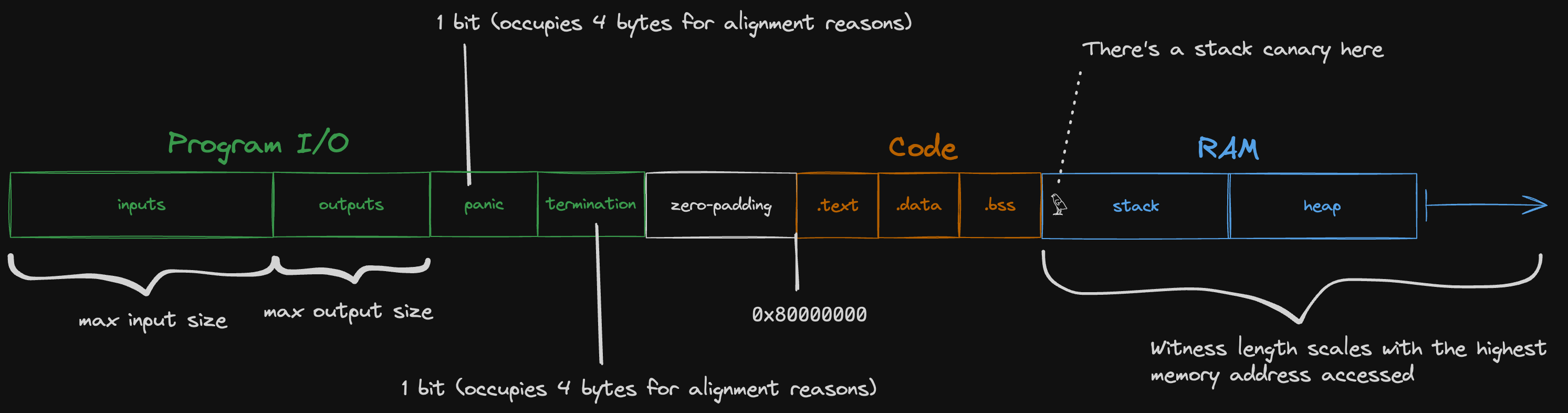
For the purposes of the memory checking argument, we remap the memory address to a witness index:
#![allow(unused)]
fn main() {
(address - memory_layout.lowest_address) / 8
}
where lowest_address is the left-most address depicted in the diagram above.
The division by eight reflects the fact that we treat guest memory as "doubleword-addressable" for the purposes of memory-checking.
Any load or store instructions that access less than a full doubleword (e.g. LB, SH, LW) are expanded into inline sequences that use the LD or SD instead.
Deviations from the Twist algorithm as described in the paper
Our implementation of the Twist prover algorithm differs from the description given in the Twist and Shout paper in a couple of ways. One such deviation is wv virtualization. Other, RAM-specific deviations are described below.
Single operation per cycle
The Twist algorithm as described in the paper assumes one read and one write per cycle, with corresponding polynomials (read address) and (write address). However, in the context of the RV64IMAC instruction set, only a single memory operation -- either a read or a write (or neither) -- is performed per cycle. Thus, a single polynomial (merging and ) suffices, simplifying and optimizing the algorithm. This polynomial is referred to as for the rest of this document.
No-op cycles
Many instructions do not access memory, so we represent them using a row of zeros in the polynomial rather than the one-hot encoding of the accessed address. Having more zeros in makes it cheaper to commit to and speeds up some of the other Twist sumchecks. This modification necessitates adjustments to the Hamming weight sumcheck, which would otherwise enforce that the Hamming weight for each "row" in is 1.
We introduce an additional Hamming Booleanity sumcheck:
where is the Hamming weight polynomial, which can be virtualized using the original Hamming weight sumcheck expression:
For simplicity, these equations are presented for the case, but as described above, for RAM is dynamic and can be greater than one.
ra virtualization
In Twist as described in the paper, a higher parameter would translate to higher sumcheck degree for the read checking, write checking, and evaluation sumchecks. Moreover, is fundamentally incompatible with the local prover algorithm for the read/write checking sumchecks.
To leverage the local algorithm while still supporting , Jolt simply carries out the read checking, write checking, and evaluation sumchecks as if , i.e. with a single (virtual) polynomial.
At the conclusion of these sumchecks, we are left with claims about the virtual polynomial. Since the polynomial is uncommitted, Jolt invokes a separate sumcheck that expresses an evaluation in terms of the constituent polynomials. The polynomials are, by definition, a tensor decomposition of , so the "ra virtualization" sumcheck is the following:
Advice Inputs
The evaluation sumcheck in Twist requires both the prover and verifier to know the initial state of the lookup table. When advice inputs are present in the RAM lookup table, the verifier doesn't have direct access to these values. To address this, the prover provides evaluations of the advice inputs and later proves their correctness against commitments held by the verifier.
For trusted advice, the commitment is generated externally; for untrusted advice, the prover generates the commitment. All advice inputs are placed at the lowest addresses of the RAM lookup table, with the larger advice type placed first to minimize field multiplications during verification.
We represent advice inputs and the RAM lookup table as multi-linear polynomials, assuming their sizes are powers of two.
Let:
- be the prover's RAM lookup table polynomial (including advice)
- be the verifier's RAM lookup table polynomial (zeros in advice section, otherwise identical to prover's)
- be the trusted advice polynomial
- be the untrusted advice polynomial
where (if this condition isn't met, we reorder the advice types to ensure the larger one comes first).
Let be the position of the single set bit in within its -bit representation. This position corresponds to bit when , or when .
The relationship between these polynomials is:
Since the verifier only needs to evaluate at a random point, it can compute this value efficiently using and the evaluations of the trusted and untrusted components.
Example
Consider a concrete example with:
- Total memory: 8192 elements ()
- Trusted advice: 1024 elements ()
- Untrusted advice: 128 elements ()
The memory layout would be:
- Addresses with the 3 MSBs as
000: trusted advice region (all combinations of the remaining 10 bits) - Addresses with the MSBs as
001000: untrusted advice region (all combinations of the remaining 7 LSBs)
This arrangement minimizes verifier computation. If we placed untrusted advice first, the verifier would need to check multiple bit patterns (000001, 000010, etc.) for the trusted section, resulting in significantly more field multiplications.
Output Check
Jolt ensures correctness of guest program outputs via the output check sumcheck. Guest I/O operations, including outputs, inputs, and termination or panic bits, occur within a designated memory region. At execution completion, outputs and relevant status bits are written into this region.
Verifying that the claimed outputs and status bits are correct amounts to checking that the following polynomials agree at the indices corresponding to the program I/O memory region:
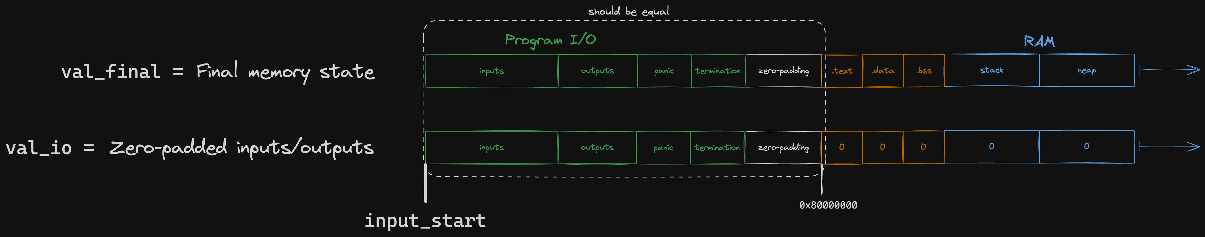
Note that val_io is only contains information known by the verifier.
To check that these two polynomials are equal, we use the following sumcheck:
where is a "range mask" polynomial, equal to 1 at all the indices corresponding to the program I/O region and 0 elsewhere. The MLE for a range mask polynomial that isolates the range can be written as follows:
It is implemented in code as RangeMaskPolynomial.
This output check sumcheck generates a claim about the final memory state polynomial (), which, being virtual, is proven using the evaluation sumcheck:
Intuitively, the delta between the final and initial state of some memory cell is the sum of all increments to that cell.
The verifier also requires evaluations of the advice sections to compute . As with the evaluation described above, the prover provides these evaluations. Since both sumchecks use the same randomness, the prover only needs to provide one evaluation proof per advice type. If different randomness were used, separate proofs would be required for each sumcheck.
You may have noticed in the above expression that if a polynomial only over cyclce variables, while the book describes . This change is explained in wv virtualization.
Both the and evaluation sumchecks use the virtual polynomial, with claims subsequently proven via ra virtualization sumcheck.
Instruction execution
One distinguishing feature of Jolt among zkVM architectures is how it handles instruction execution, i.e. proving the correct input/output behavior of every RISC-V instruction in the trace. This is primarily achieved through the Shout lookup argument.
Large Lookup Tables and Prefix-Suffix Sumcheck
The Shout instance for instruction execution must query a massive lookup table -- effectively of size , since the lookup query is constructed from two 64-bit operands. This parameter regime is discussed in the Twist and Shout paper (Section 7), which proposes the use of sparse-dense sumcheck. However, upon implementation it became clear that sparse-dense sumcheck did not generalize well to the full RISC-V instruction set.
Instead, Jolt introduces a new algorithm: prefix-suffix sumcheck, described in the appendix of Proving CPU Executions in Small Space. Like the sparse-dense algorithm, it requires some structure in the lookup table:
- The lookup table must have an MLE that is efficiently evaluable by the verifier. The
JoltLookupTabletrait encapsulates this MLE. - The lookup index can be split into a prefix and suffix, such that MLEs can be evaluated independently on the two parts and then recombined to obtain the desired lookup entry.
- Every prefix/suffix MLE is efficiently evaluable (constant time) on Boolean inputs
The prefix-suffix sumcheck algorithm can be conceptualized as a careful application of the distributive law to reduce the number of multiplications required for a sumcheck that would otherwise be intractably large.
To unpack this, consider the read-checking sumcheck for Shout, as presented in the paper.
Naively, this would require multiplications, which is far too large given and . But suppose has prefix-suffix structure. The key intuition of prefix-suffix structure is captured by the following equation:
You can think of and as the high-order and low-order "bits" of , respectively, obtained by splitting at some partition index. The PrefixSuffixDecomposition trait specifies which prefix/suffix MLEs to evaluate and how to combine them.
We will split eight times at eight different indices, and these will induce the eight phases of the prefix-suffix sumcheck. Each of the eight phases encompasses 16 rounds of sumcheck (i.e. 16 of the address variables ), so together they comprise the first rounds of the read-checking sumcheck.
Given our prefix-suffix decomposition of , we can rewrite our read-checking sumcheck as follows:
Note that we have replaced with just . Since is degree 1 in each variable, we will treat it as a single multilinear polynomial while we're binding those variables (the first rounds). The equation as written above depicts the first phase, where is the first 16 variables of , and is the last 112 variables of .
Rearranging the terms in the sum, we have:
Note that the summand is degree 2 in , the variables being bound in the first phase:
- appears in
- also appears in appears in the paranthesized expression in
Written in this way, it becomes clear that we can treat the first 16 rounds as a mini-sumcheck over just the 16 variables, and with just multilinear terms. If we can efficiently compute the coefficients of each mulitlinear term, the rest of this mini-sumcheck is efficient. Each evaluation of can be computed in constant time, so that leaves the parenthesized term:
This can be computed in : since is one-hot, we can do a single iteration over and only compute the terms of the sum where . We compute a table of evaluation a priori, and can be evaluated in constant time on Boolean inputs.
After the first phase, the high-order 16 variables of will have been bound. We will need to use a new sumcheck expression for the next phase:
Now are random values that the first 16 variables were bound to, and are the next 16 variables of . Meanwhile, now represents the last 96 variables of .
This complicates things slightly, but the algorithm follows the same blueprint as in phase 1. This is a sumcheck over the 16 variables, and there are two multilinear terms. We can still compute each evaluation of in constant time, and we can still compute the parenthesized term in time (observe that there is exactly one non-zero coefficient of per cycle ).
After the first rounds of sumcheck, we are left with:
which we prove using the standard linear-time sumcheck algorithm. Note that here is a virtual polynomial.
Prefix and Suffix Implementations
Jolt modularizes prefix/suffix decomposition using two traits:
SparseDensePrefix(underprefixes/)SparseDenseSuffix(undersuffixes/)
Each prefix/suffix used in a lookup table implements these traits.
Multiplexing Between Instructions
An execution trace contains many different RISC-V instructions.
Note that there is a many-to-one relationship between instructions and lookup tables -- multiple instructions may share a lookup table (e.g., XOR and XORI).
To manage this, Jolt uses the InstructionLookupTable trait, whose lookup_table method returns an instruction's associated lookup table, if it has one (some instructions do not require a lookup).
Boolean lookup table flags indicate which table is active on a given cycle. At most one flag is set per cycle. These flags allow us to "multiplex" between all of the lookup tables:
where the sum is over all lookup tables .
Only one table's flag is 1 at any given cycle , so only that table's contributes to the sum.
This term becomes a drop-in replacement for as it appears in the Shout read-checking sumcheck:
Note that each here has prefix-suffix structure.
raf Evaluation
The -evaluation sumcheck in Jolt deviates from the description in the Twist/Shout paper. This is mostly an artifact of the prefix-suffix sumcheck, which imposes some required structure on the lookup index (i.e. the "address" variables ).
Case 1: Interleaved operands
Consider, for example, the lookup table for XOR x y.
Intuitively, the lookup index must be crafted from the bits of x and y.
A first attempt might be to simply concatenate the bits of x and y, i.e.:
Unfortunately, there is no apparent way for this formulation to satisfy prefix-suffix structure.
Instead we will interleave the bits of x and y, i.e.
With this formulation, the prefix-suffix structure is easily apparent. Suppose the prefix-suffix split index is 16, so:
Then XOR x y has the following prefix-suffix decomposition:
By inspection, effectively computes the 8-bit XOR of the high-order bits of x and y, while computes the 56-bit XOR of the low-order bits of x and y.
Then the full result XOR x y is obtained by concatenating (adding) the two results.
Now that we've confirmed that we have something with prefix-suffix structure, we can write down the -evaluation sumcheck expression.
Instead of a single polynomial, here we have two lookup operands x and y, which are called LeftLookupOperand and RightLookupOperand in code.
These are the values that appear in Jolt's R1CS constraints.
The point of the -evaluation sumcheck is to relate these (non-one-hot) polynomials to their one-hot counterparts.
In the context of instruction execution Shout, this means the polynomial.
Since we have two -like polynomials, we have two sumcheck instances:
This captures the interleaving behavior we described above: LeftLookupOperand is the concatenation of the "odd bits" of , while RightLookupOperand is the concatenation of the "even bits" of .
Case 2: Single operand
Many RISC-V instructions are similar to XOR, in that interleaving the operand bits lends itself to prefix-suffix structure.
However, there are some instructions where this is not the case.
The execution of some arithmetic instructions, for example, are handled by computing the corresponding operation in the field, and applying a range-check lookup to the result to truncate potential overflow bits.
In this case, the lookup index corresponds to the (single) value y being range-checked, so we do not interleave its bits with another operand.
Instead, we just have:
In this case, we have the following sumchecks:
LeftLookupOperand is 0 and RightLookupOperand will be the concatenation of all the bits of .
In order to handle Cases 1 and 2 simultaneously, we can use the same "multiplexing" technique as in the read-checking sumcheck. We use a flag polynomial to indicate which case we're in:
where , , and are circuit flags.
Prefix-suffix structure
These sumchecks have similar structure to the read-checking sumcheck. A side-by-side comparison of the read-checking sumcheck with the sumchecks for Case 1:
As it turns out, and have prefix-suffix structure, so we can also use the prefix-suffix algorithm for these sumchecks. Due to their similarities, we batch the read-checking and these -evaluation sumchecks together in a bespoke fashion.
Other sumchecks
ra virtualization
The lookup tables used for instruction execution are of size , so we set as our decomposition parameter such that .
Similar to the RAM Twist instance, we opt to virtualize the polynomial. In other words, Jolt simply carries out the read checking and evaluation sumchecks as if .
At the conclusion of these sumchecks, we are left with claims about the virtual polynomial. Since the polynomial is uncommitted, Jolt invokes a separate sumcheck that expresses an evaluation in terms of the constituent polynomials. The polynomials are, by definition, a tensor decomposition of , so the " virtualization" sumcheck is the following:
Since the degree of this sumcheck is , using the standard linear-time sumcheck prover algorithm would make this sumcheck relatively slow. However, we employ optimizations specific to high-degree sumchecks, adapting techniques from the Karatsuba and Toom-Cook multiplication algorithms.
One-hot checks
Jolt enforces that the polynomials used for instruction execution are one-hot, using a Booleanity and Hamming weight sumcheck as described in the paper. These implementations follow the Twist and Shout paper closely, with no notable deviations.
Bytecode
At each cycle of the RISC-V virtual machine, the current instruction (as indicated by the program counter) is "fetched" from the bytecode and decoded. In Jolt, this is proven by treating the bytecode as a lookup table, and fetches as lookups. To prove the correctness of these lookups, we use the Shout lookup argument.
One distinguishing feature of the bytecode Shout instance is that we have multiple instances of the read-checking and -evaluation sumchecks. Intuitively, the bytecode serves as the "ground truth" of what's being executed, so one would expect many virtual polynomial claims to eventually lead back to the bytecode. And this holds in practice –– in the Jolt sumcheck DAG diagram, we see that there are five stages of read-checking claims pointing to the bytecode read-checking node, and two evaluation claims folded into stages 1 and 3.
Each stage has its own unique opening point, so having in-edges of different colors implies that multiple instances of that sumcheck must be run in parallel to prove the different claims.
Read-checking
Another distinguishing feature of the bytecode Shout instance is that we treat each entry of lookup table as containing a tuple of values, rather than a single value. Intuitively, this is because each instruction in the bytecode encodes multiple pieces of information: opcode, operands, etc.
The figure below loosely depicts the relationship between bytecode and polynomial.
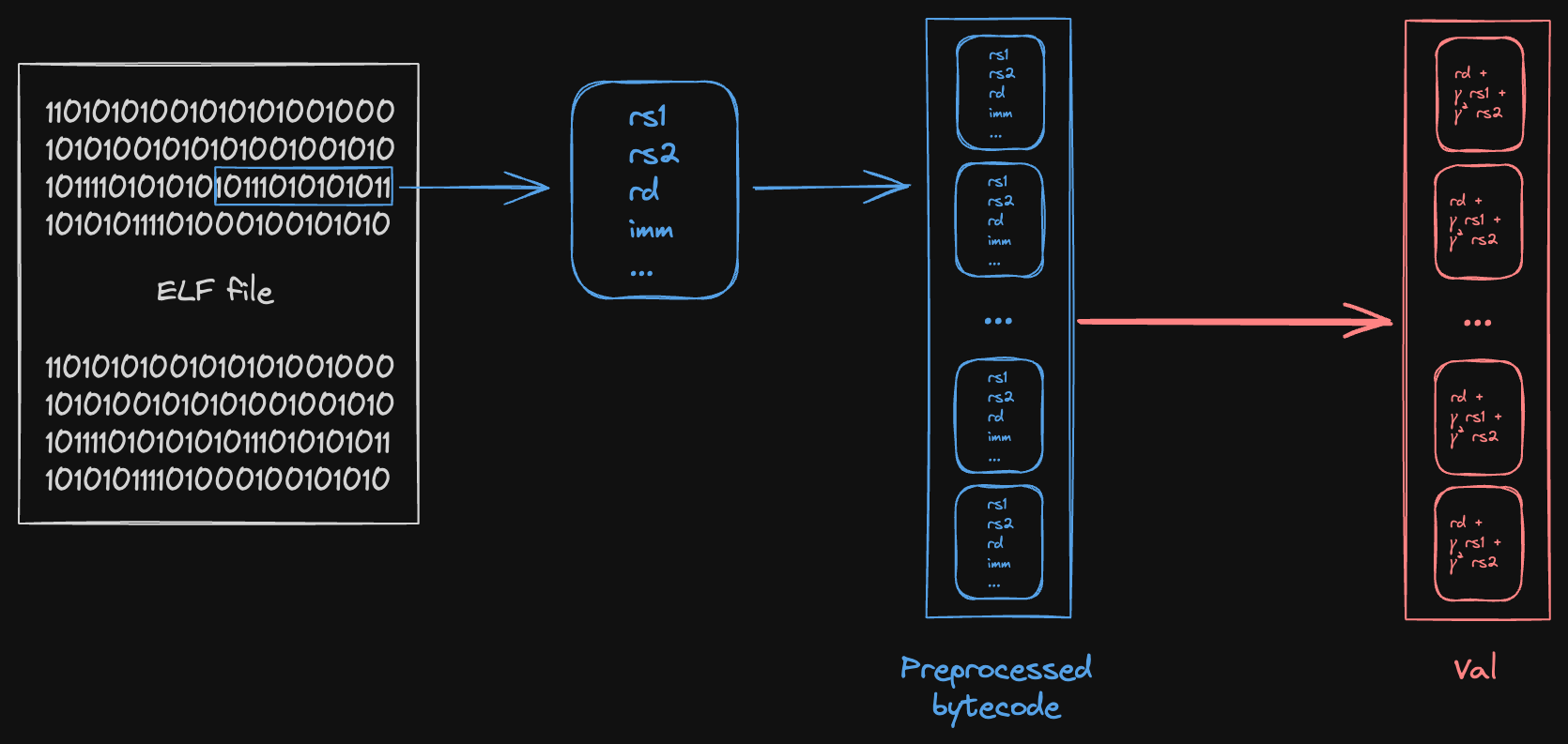
We start from some ELF file, compiled from the guest program. For each instruction in the ELF (raw bytes), we decode/preprocess the instruction into a structured format containing the individual witness values used in Jolt:
Then, we compute a Reed-Solomon fingerprint of some subset of the values in the tuple, depending on what claims are being proven. These fingerprints serve as the coefficients of the polynomial for that read-checking instance.
-evaluation
-evaluation claims for the program counter are folded into the multi-stage read-checking sumcheck rather than being handled separately. There are two claims:
- raf claim 1: From the Spartan "outer" sumcheck, folded into Stage 1 with weight
- raf claim 3: From the Spartan "shift" sumcheck, folded into Stage 3 with weight
The polynomial in the context of bytecode is the expanded program counter (), which maps each cycle to the bytecode index being executed. This is distinct from , which is the ELF/memory address.
Batching read-checking and -evaluation together
The bytecode read-checking sumcheck combines claims from five different sumcheck stages into a single batched sumcheck, using two levels of random linear combinations (RLCs):
- Stage-level RLC (using ): Combines the five stages together
- Per-stage RLC (using ): Combines multiple claims within each stage
The five stages are:
- Stage 1: Spartan outer sumcheck claims (program counter, immediate values, circuit flags)
- Stage 2: Product virtualization claims (jump/branch flags, register write flags)
- Stage 3: Shift sumcheck claims (instruction operand flags, virtual instruction metadata)
- Stage 4: Register read-write checking claims (register addresses)
- Stage 5: Register value evaluation and instruction lookup claims (register addresses, lookup table flags)
Additionally, bytecode claims for the program counter are folded into stages 1 and 3.
Combined Sumcheck Expression
The overall sumcheck proves the following identity:
where:
- ranges over bytecode indices (address space)
- ranges over cycle indices (time dimension)
- is the read access polynomial indicating cycle accesses bytecode row
- is the stage-specific value polynomial encoding instruction data
- is the identity polynomial that converts a bytecode index from binary form to the corresponding field element (used for claims)
- is the multilinear indicator for
- is the multilinear indicator for , where is the bytecode index of the ELF entry point
- is the stage-folding challenge
- challenges are used within each to combine multiple sub-claims
Note that the claims treat the expanded program counter as , not UnexpandedPC.
Entry-point constraint
The term enforces that execution begins at the ELF entry point. Both prover and verifier add unconditionally to the left-hand side. An honest trace satisfies , so the new right-hand side term also sums to . If the committed trace starts at any other instruction, the sumcheck fails. No additional opening proof is required — the term reduces to the same opening point as the rest of the sumcheck.
Stage Polynomials
Each of the five claims has a corresponding polynomial that encodes different instruction properties. Using per-stage challenges , these are defined as:
Stage 1 (Spartan outer sumcheck):
Stage 2 (Product virtualization):
Stage 3 (Shift sumcheck):
Stage 4 (Register read-write checking):
Stage 5 (Register value evaluation and instruction lookups):
where:
- is the instruction's ELF/memory address (not the bytecode index )
- equals 1 if instruction has destination register , and 0 otherwise (similarly for and )
- Various boolean flags indicate instruction properties
Instruction address
Each instruction in the bytecode has two associated "addresses":
- Bytecode index : its index in the expanded bytecode. "Expanded" bytecode refers to the preprocessed bytecode, after instructions are expanded to their virtual sequences. This is what the polynomial uses to indicate which bytecode row is accessed.
- ELF/memory address : its memory address as given by the ELF. All the instructions in a virtual sequence are assigned the address of the "real" instruction they were expanded from. This is stored as part of the instruction data in bytecode row .
The bytecode index is used for addressing within the sumcheck (the variable in the double sum). The ELF address is used to enforce program counter updates in the R1CS constraints, and is treated as a part of the tuple of values in the preprocessed bytecode.
The "outer" and shift sumchecks in Spartan output claims about the virtual UnexpandedPC polynomial, which corresponds to the ELF address. These claims are proven using bytecode read-checking (specifically, they appear in the Stage 1 and Stage 3 value polynomials).
Flags
There are two types of Boolean flags used in Jolt:
- Circuit flags, used in R1CS constraints
- Lookup table flags, used in the instruction execution Shout
The associated flags for a given instruction in the bytecode can be computed a priori (i.e. in preprocessing), so any claims about these flags arising from Spartan or instruction execution Shout are also proven using bytecode read-checking. Circuit flags appear in Stages 1, 2, and 3, while lookup table flags appear in Stage 5.
Sumcheck Structure and Binding Order
The bytecode read-checking sumcheck proceeds in two phases:
Phase 1: Address Variables (first rounds)
In the first rounds, address variables are bound in low-to-high order. During this phase:
- The polynomials for each stage are bound, eventually reducing to scalar values
- Intermediate "F" polynomials are computed: , representing the weighted frequency that each bytecode row is accessed
- These F polynomials are also bound during the address phase
The sumcheck univariate in this phase has degree 2 (quadratic).
Phase 2: Cycle Variables (final rounds)
In the final rounds, cycle variables are bound, also in low-to-high order. During this phase:
- The polynomial is computed as a product of chunked one-hot polynomials:
- Each stage uses a
GruenSplitEqPolynomialto efficiently handle the per-stage evaluations - The bound and values from Phase 1 are used as coefficients
The sumcheck univariate in this phase has degree .
The chunking parameter is chosen based on the bytecode size to balance prover time and proof size. Larger reduces the number of committed RA polynomials but increases the degree (and thus the cost per round) of the sumcheck.
One-hot checks
Jolt enforces that the polynomials used for bytecode Shout are one-hot, using a Booleanity and Hamming weight sumcheck as described in the paper. These implementations follow the Twist and Shout paper closely, with no notable deviations.
Batched opening proof
The final stage (stage 8) of Jolt is the batched opening proof.
Over the course of the preceding stages, we obtain polynomial evaluation claims that must be proven using the polynomial commitment scheme's opening proof.
Instead of proving these openings "just-in-time", we accumulate them and defer the opening proof to the last stage (see ProverOpeningAccumulator and VerifierOpeningAccumulator for how this accumulation is implemented).
By waiting until the end, we can batch-prove all of the openings, instead of proving them individually.
This is important because the Dory opening proof is relatively expensive for the prover, so we want to avoid doing it multiple times.
Claim reduction sumchecks
Throughout the earlier stages of Jolt, various components generate multiple polynomial evaluation claims that need to be consolidated before the final opening proof. Conceptually, claim reduction sumchecks are instantiation of the "Multiple polynomials, multiple points" subprotocol.
These claim reduction sumchecks serve two purposes:
- Reduce the number of claims that need to be virtualized by a subsequent sumcheck. E.g. if the same virtual polynomial is opened at two different points and , a claim reduction can be applied to avoid running two instances of the sumcheck that virtualized .
- Reduce the number of claims that need to be proven via PCS opening proof. While we can leverage the homomorphic properties of Dory in the Multiple polynomials, same point subprotocol, we must first reduce multiple opening points to a single, unified opening point.
The claim reduction sumchecks can be found in crates/jolt-prover-legacy/src/zkvm/claim_reductions/ and include:
- Instruction lookups (
instruction_lookups.rs): Aggregates instruction lookup claims (lookup outputs and operands) from Spartan. - Registers (
registers.rs): Reduces register read/write claims (rd, rs1, rs2) from Spartan. - RAM RA (
ram_ra.rs): Consolidates the four RAM read-address (RA) claims from various RAM-related sumchecks (raf evaluation, read-write checking, Val evaluation, Val-final evaluation) into a single claim for the RA virtualization sumcheck. - Increments (
increments.rs): Reduces claims related to increment checks. - Hamming weight (
hamming_weight.rs): Reduces hamming weight-related claims. - Advice (
advice.rs): Reduces claims from advice polynomials. - Bytecode (
bytecode.rs): Reduces committed bytecode openings into the shared Stage 8 final opening layout. - Program image (
program_image.rs): Reduces the committed initial-memory image into the same final opening layout.
How claim reduction sumchecks work
A claim reduction sumcheck takes multiple polynomial evaluation claims, potentially at different evaluation points, and consolidates them into a single claim (or fewer claims) using the sumcheck protocol. The general pattern is:
- Input: Multiple polynomial evaluation claims of the form
- Batching: Random challenge is sampled from the transcript to batch the claims together
- Sumcheck: Prove a sumcheck identity of the form:
- Output: Polynomial evaluation claims of the form for a single, unified point derived from the sumcheck challenges.
Final reduction
After the claim reduction sumchecks have consolidated related claims, we perform a final reduction to prepare for the Dory opening.
We apply the Multiple polynomials, same point subprotocol to reduce the claims to a single claim, namely the evaluation of an RLCPolynomial representing a random linear combination of all the opened polynomials.
On the verifier side, this entails taking a linear combination of commitments. Since Dory is an additively homomorphic commitment scheme, the verifier is able to do so.
Precommitted polynomials and final opening layout
Most Stage 8 polynomials are trace-domain polynomials: their shape is determined by the padded execution trace and the address domain. Some committed polynomials, however, are fixed independently of the trace. Examples include bytecode chunks, the program image, and trusted or untrusted advice. In the implementation these independently committed objects are called precommitted polynomials.
The goal of Stage 8 is still the same: every committed polynomial should be opened at one batched Dory proof. The subtlety is that a precommitted polynomial keeps the Dory matrix shape it had when it was committed, while the trace-domain polynomials use Jolt's native trace layout.
We use the following terminology:
- Native trace layout: the Dory layout induced by trace-domain polynomials, with variables.
- Embedded precommitted polynomial: a precommitted polynomial whose committed Dory matrix fits inside the native trace layout. It is embedded by top-left zero padding.
- Dominant precommitted polynomial: a precommitted polynomial that is larger than the native trace layout. It determines an enlarged final opening layout.
- Final opening layout: the Dory matrix used by the single Stage 8 opening proof. This is the native trace layout when no dominant precommitted polynomial exists, and the enlarged layout otherwise.
In this section we write:
- for the number of cycle variables, i.e. the log trace length
- for the number of address variables, i.e. the log address-space size
- for the number of extra variables contributed by the dominant precommitted polynomial beyond the native trace layout
With that notation, the final opening layout has
Equivalently, Stage 8 works in a Dory matrix of size where
Here is the number of row variables and is the number of column variables. This matches the implementation in DoryGlobals::balanced_sigma_nu() and the split used by PrecommittedClaimReduction::project_dory_round_permutation_for_poly().
The native trace layout is the special case . The design constraint is that dominant precommitted polynomials should not force the earlier trace-domain sumchecks to run over a padded trace. So Jolt schedules the final-opening reductions as follows:
- the cycle stage (Stage 6b) has exactly rounds
- the address stage (Stage 7) has exactly rounds
- precommitted reductions are forward-loaded so they see the extra dominant coordinates
- native trace-domain reductions are backward-loaded so their old round scheduling is preserved
This keeps trace-domain work native through the earlier stages and leaves Stage 8 with only one normalization problem: all produced opening points must be interpreted inside the final opening layout.
If some precommitted polynomial already has variables, we call it a dominant precommitted polynomial. Otherwise there is no dominant precommitted polynomial, , and the final opening layout is just the native trace layout.
How Native Polynomials Sit In The Final Layout
Native trace-domain polynomials are placed in the final opening layout according to the Dory layout. As a concrete example, take . Since Dory uses a balanced split, this means:
so the final Dory matrix has rows and columns, for a total of slots.
CycleMajor dense placement
Take a dense polynomial with variables and coefficients
In CycleMajor, the dense polynomial is written across the top of the final matrix, so only the lowest index bits vary:
Final 4 x 8 matrix

          col000   col001   col010   col011   col100   col101   col110   col111
row00   | a_000  | a_001  | a_010  | a_011  | a_100  | a_101  | a_110  |  a_111 |
row01   |    .   |    .   |    .   |    .   |    .   |    .   |    .   |    .   |
row10   |    .   |    .   |    .   |    .   |    .   |    .   |    .   |    .   |
row11   |    .   |    .   |    .   |    .   |    .   |    .   |    .   |    .   |
so the first bits are fixed and only the last bits vary.
AddressMajor dense placement
Now take the same final opening layout , but the dense polynomial should use the highest bits. Then its coefficients are written into slots whose last bits are zero:
In the same matrix this looks like:
Final 4 x 8 matrix

          col000   col001   col010   col011   col100   col101   col110   col111
row00   | a_000  |    .   |    .   |    .   | a_001  |    .   |    .   |    .   |
row01   | a_010  |    .   |    .   |    .   | a_011  |    .   |    .   |    .   |
row10   | a_100  |    .   |    .   |    .   | a_101  |    .   |    .   |    .   |
row11   | a_110  |    .   |    .   |    .   | a_111  |    .   |    .   |    .   |
The same idea applies to one-hot polynomials:
- in
CycleMajor, they use the lowest bits - in
AddressMajor, they use the highest bits, so the trailing bits are zero
When Address-Major Dense Stride Exceeds The Row Width
In AddressMajor, dense polynomials are embedded with stride . Sometimes that stride is larger than the number of columns of the final Dory matrix. This is the special branch handled in dory/wrappers.rs.
Take a real example:
- final opening layout , so the balanced Dory matrix is
- dense polynomial has variables, so it has 4 coefficients
- therefore , so the stride is
Since the row width is only 16, consecutive coefficients jump by two whole rows:
coeff a_00 -> slot  0 -> row 0, col 0
coeff a_01 -> slot 32 -> row 2, col 0
coeff a_10 -> slot 64 -> row 4, col 0
coeff a_11 -> slot 96 -> row 6, col 0
and the matrix picture is:
8 x 16 final matrix

row0  | a_00  .  .  .  .  .  .  .  .  .  .  .  .  .  .  . |
row1  |  .    .  .  .  .  .  .  .  .  .  .  .  .  .  .  . |
row2  | a_01  .  .  .  .  .  .  .  .  .  .  .  .  .  .  . |
row3  |  .    .  .  .  .  .  .  .  .  .  .  .  .  .  .  . |
row4  | a_10  .  .  .  .  .  .  .  .  .  .  .  .  .  .  . |
row5  |  .    .  .  .  .  .  .  .  .  .  .  .  .  .  .  . |
row6  | a_11  .  .  .  .  .  .  .  .  .  .  .  .  .  .  . |
row7  |  .    .  .  .  .  .  .  .  .  .  .  .  .  .  .  . |
So the logical embedding is unchanged, but it is no longer a convenient row-local chunking. Because polynomial lengths are powers of two, the placement still stays aligned: either the stride is a multiple of the row width, so the polynomial occupies the same column range in every row it touches, or the stride divides the row width, so it stays in a fixed column but appears only in every few rows, as in the example above.
Final Dory Opening Point
In summary
- in
CycleMajor, the native dense / one-hot layout consumes the low bits of the final Dory point, so any extra precommitted variables must sit on the high side - in
AddressMajor, the native layout consumes the high bits, so any extra precommitted variables must sit on the low side - each block appears in reverse because we always bind polynomials during claim reduction sumchecks from low to high bits
Now we study two cases: If there is a dominant precommitted polynomial, let the raw cycle-stage challenges be
and the raw address-stage challenges be
The final big-endian Dory opening point is obtained by normalizing these challenges into Dory order.
For AddressMajor:
For CycleMajor:
Each block is reversed, and the extra variables move to different sides depending on the layout.
If there is no dominant precommitted polynomial, then the final point is anchored by the ordinary native openings:
- in this case the final opening layout is just the native trace layout, so
- let be the cycle-stage opening point from
IncClaimReduction - let be the full opening point from
HammingWeightClaimReduction, decomposed as where has length
These are already normalized opening points. In CycleMajor, compute_final_opening_point() checks that the IncClaimReduction opening point agrees with the native cycle suffix . When there are no extra dominant coordinates, this means .
Then:
For AddressMajor:
For CycleMajor:
The implementation is located in compute_final_opening_point() in crates/jolt-prover-legacy/src/zkvm/mod.rs.
Embedded Precommitted Polynomials
The verifier already has the commitment to an embedded precommitted polynomial. That commitment is computed under the convention that the polynomial occupies the top-left block of its own balanced Dory matrix, meaning the earliest rows and earliest columns. So when we embed that polynomial into the final opening layout, we must preserve that same top-left placement; otherwise the verifier would be checking the Dory proof against a different layout from the one encoded in the commitment.
Final Dory matrix: 2^nu_D rows x 2^sigma_D columns
Smaller precommitted matrix: 2^nu_C rows x 2^sigma_C columns

                    left 2^sigma_C cols         remaining cols
                 +---------------------------+------------------+
top 2^nu_C rows  | smaller precommitted poly | not used by this |
                 |        lives here         |      poly        |
                 +---------------------------+------------------+
remaining rows   | not used by this poly     | not used by this |
                 |                           |      poly        |
                 +---------------------------+------------------+
Suppose the smaller precommitted polynomial has
variables, while the final point has
Split the final point as
where:
- has length
- has length
- has length
- has length
Then the smaller polynomial is evaluated on
The reason is that top-left embedding forces the missing high row bits and high column bits to be zero:
final row variables : [row_hi | row_lo]
final col variables : [col_hi | col_lo]

top-left embedding forces:
  row_hi = 0
  col_hi = 0
So if is the smaller polynomial and is its embedding into the final matrix, then
The same selector appears when the final RLCPolynomial mixes a native trace-domain polynomial with an embedded precommitted polynomial:
Permuting Precommitted Polynomial Variables
The precommitted sumchecks still bind variables low-to-high. But the final Dory point order is determined by the final opening layout, not by the order in which those rounds happen.
So Jolt permutes the variables of each precommitted polynomial before running the sumcheck. This keeps the sumcheck code simple while ensuring the final claim corresponds to the original polynomial at the correct Stage 8 point. This permutation is cheap because it is only a variable-position movement, so on the coefficient table it is just a bit permutation of the Boolean-hypercube evaluations.
Here is a concrete 3-variable example. Suppose the original polynomial is encoded by
point       000  001  010  011  100  101  110  111
P(point)     v0   v1   v2   v3   v4   v5   v6   v7
Now suppose the final opening layout wants the variables in the order rather than . Define
Then the new coefficient table becomes
point        000  001  010  011  100  101  110  111
P'(point)     v0   v4   v2   v6   v1   v5   v3   v7
because
P'(000) = P(000)
P'(001) = P(100)
P'(010) = P(010)
P'(011) = P(110)
P'(100) = P(001)
P'(101) = P(101)
P'(110) = P(011)
P'(111) = P(111)
After the sumcheck finishes, normalize_opening_point() converts the collected challenges back into the true opening point of the original, non-permuted polynomial.
RLCPolynomial
Recall that all of the polynomials in Jolt fall into one of two categories: one-hot polynomials (the and arising in Twist/Shout), and dense polynomials (we use this to mean anything that's not one-hot).
We use the RLCPolynomial struct to represent a random linear combination (RLC) of multiple polynomials, which may include both dense and one-hot polynomials.
We handle the two types separately:
- We eagerly compute the RLC of the dense polynomials. So if there are dense polynomials, each of length in the RLC, we compute the linear combination of their coefficients and store the result in the
RLCPolynomialstruct as a single vector of length . - We lazily compute the RLC of the one-hot polynomials. So if there are one-hot polynomials, we store (coefficient, reference) pairs in
RLCPolynomialto represent the RLC. Later in the Dory opening proof when we need to compute a vector-matrix product usingRLCPolynomial, we do so by computing the vector-matrix product using the individual one-hot polynomials (as well as the dense RLC) and taking the linear combination of the resulting vectors.
Twist and Shout
🚧 These docs are under construction 🚧
👷If you are urgently interested in this specific page, open a Github issue and we'll try to expedite it.👷
One-hot polynomials
A one-hot vector of length is a unit vector in , i.e., a vector of length with exactly one entry equal to and all other entries equal to .
In Jolt, we refer to the multilinear extension (MLE) of a one-hot vector as a one-hot polynomial.
We also use the same terminology to refer to the concatenation of different one-hot vectors. For example, if where each is one-hot, then we'll call one-hot, and say the same about its MLE.
Shout
Shout is a batch-evaluation argument. Let be any function, and suppose the prover has already committed to inputs to . A batch-evaluation argument gives the verifier query access to the MLE of the output vector .
From the verifier's perspective, a batch-evaluation argument is an efficient reduction from the difficult task of evaluating the MLE of the output vector at a random point, to the easier task of evaluating the MLE of the input vector at a random point.
In Shout, a wrinkle is that each input to is committed in one-hot form (i.e., as a unit vector in ) rather than as a binary vector in . For example, if , , and , then in Shout will be committed as the length-four unit vector while will be committed as .
Let denote the evaluation table of , i.e., is the vector of length whose 'th entry stores . Let denote the matrix whose 'th row is the one-hot representation of vector .
Then is simply the inner product of row of with . This can be seen to imply that for any ,
All that Shout does is apply the sum-check protocol to compute the above sum. From the verifier's perspective, this reduces the task of computing to that of evaluation at a random point and evaluation at a random point. Since the vector was committed by the prover, the prover can provide the requested evaluation of along with an evaluation proof.
In the case where committing to, or providing an evaluation proof for, is too expensive, Shout instead virtualizes . This means itself is not committed. Rather, several smaller vectors are committed, and when the verifier needs to evaluate at a random point, the sum-check protocol is applied to reduce evaluating (the MLE of) at a point to evaluating (the MLEs of) the simpler vectors at a different point.
In Shout, this virtualization uses the fact that, since (each of the rows of) is one-hot and of length , (each row of) can be expressed as the tensor product of smaller one-hot vectors, each of length . Rather than committing to directly, the prover commits to the smaller vectors, and then we use an additional application of the sum-check protocol to reduce the task of evaluating at a point to the task of evaluation each of the smaller vectors at a point.
Prefix-suffix Shout
For the Shout verifier to be fast, all that is needed is that be quickly evaluable. This is the case for all of the primitive RISC-V instructions (and many other functions). However, for the Shout prover to be fast, needs additional structure. We call the kind of structure exploited to make the Jolt prover fast prefix-suffix structure. Prefix-suffix structure is spiritually similar to the notion of decomposable tables in Lasso: roughly, it captures the situation where a single evaluation of at input can be obtained by splitting into chunks each of size , evaluating a simple function on each chunk, and putting the evaluations together in a simple way. Whereas the Lasso prover had to explicitly commit to the chunks, the Shout prover only uses the decomposition ``in its own head'' to compute its sum-check messages quickly. This is one reason the Shout protocol is much more efficient than the Lasso protocol: table decompositions are not baked into the protocol itself but rather used only by the prover to quickly compute sum-check messages. The protocol itself is agnostic to the decomposition used (and in particular does not force the prover to use a particular decomposition).
For details, see Appendix A of [NTZ25].
Twist
Shout is a batch-evaluation argument, which can equivalently be viewed as a lookup argument, i.e., for performing reads into a read-only memory. The relevant read-only memory for Shout is the memory that stores all $2^n$ evaluations of the function $f$ being evaluated.
Twist is an extension from read-only memory to read-write memory.
Imagine the prover has already committed to $T$ read addresses and $T$ write addresses, each address indexing into a memory of size $K$. The prover has also committed to a \emph{value} associated with each write operation. We think of reads and writes as proceeding in ``cycles'' (analogous to CPU cycle), where in each cycle , the 'th read operation happens, followed by the 'th write operation.
The goal of Twist is to give the verifier query access to (the MLE of) the vector of read-values, where denotes the value returned by the 'th read operation (i.e., the value that, as of time , was most recently written to the 'th read address).
In Twist, as in Shout, each address is specified in one-hot form. So we think of the read addresses as a matrix whose 'th row is the one-hot representation of the address read at cycle , and similarly for write address .
Whereas Shout involves a single invocation of the sum-check protocol (plus an additional invocation if is virtualized in terms of smaller vectors), Twist involves several invocations of the sum-check protocol. We call these the read-checking sum-check, the write-checking sum-check, and the Val-evaluation sum-check.
Prior to the start of these three invocations of the sum-check protocol, the Twist prover commits to a vector called the Increments vector, or for short. If is the cell written at cycle , then returns the difference between the value written in cycle and the stored at cell at the start of the cycle. The next section explains that once is committed, there is actually no need to commit to the write values : the 'th write value is in fact implied by the associated increment, so there is no need to commit to both.
wv virtualization
In the Twist and Shout paper (Figure 9), the read and write checking sumchecks of Twist are presented as follows:
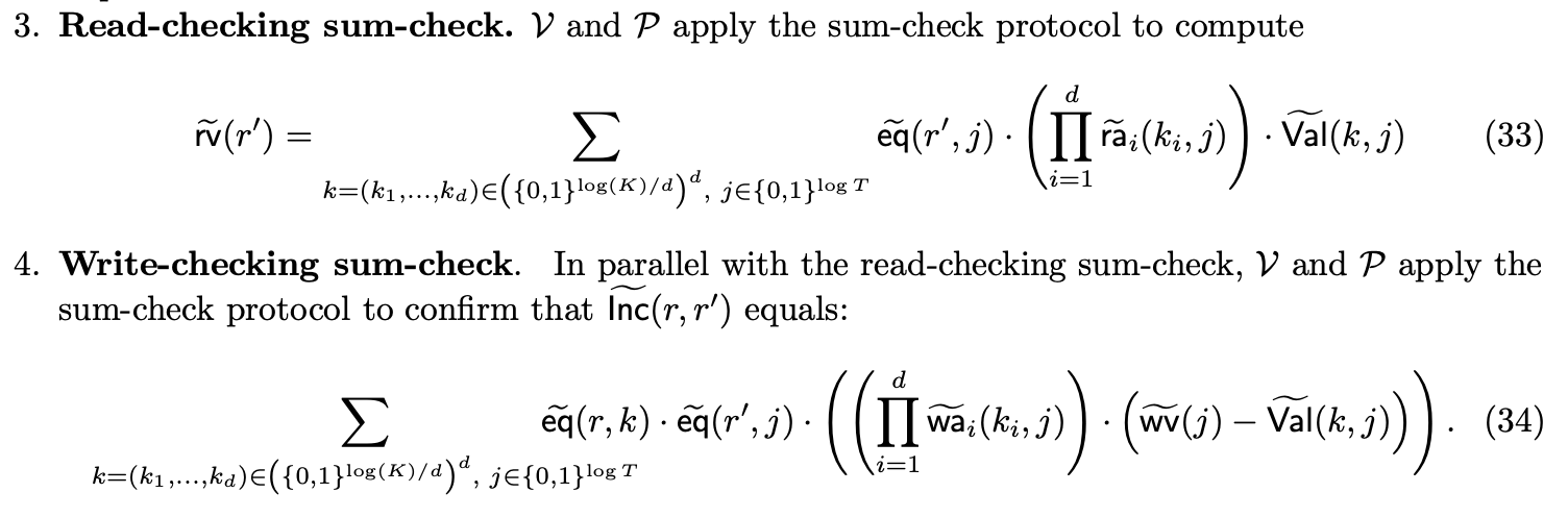
Observe that the write checking sumcheck is presented as a way to confirm that an evaluation of is correct.
Under this formulation, both and the polynomial are committed.
With a slight tweak, we can avoid committing to . First, we will modify to be a polynomial over just the cycle variables, i.e. . Intuitively, the th coefficient of is the delta for the memory cell accessed at cycle (agnostic to which cell was accessed).
Second, we will reformulate the write checking sumcheck to more closely match the read checking sumcheck:
Intuitively, the write value at cycle is equal to whatever was already in that register (), plus the increment ().
We also need to tweak the -evaluation sumcheck to accommodate the modification . As presented in the paper:
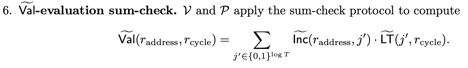
After modifying to be a polynomial over just the cycle variables:
Dory
Dory is the polynomial commitment scheme used in Jolt. It is based on the scheme described in Lee21 and implemented in the a16z/dory repository.
Background: AFGHO commitments
Dory uses a pairing-inner-product commitment to vectors of group elements, based on the structure-preserving commitment scheme of Abe-Fuchsbauer-Groth-Haralambiev-Ohkubo, 2010 (AFGHO).
Work over bilinear groups , and write the group operations additively. Given a vector of source-group elements and public generators , the core commitment is the pairing inner product:
The construction is symmetric: vectors in can be committed with generators in . A hiding version additionally adds a random multiple of a fixed target-group element, for example .
The important property for Dory is additive homomorphism. Since pairing is bilinear, commitments to source-group vectors can be linearly combined in :
For scalar polynomial coefficients, Dory first commits each row of coefficients into a element. Those row commitments then form the source-group vector that is committed with the AFGHO pairing-inner-product commitment. This is the two-tier structure that gives Dory both small commitments and efficient batched openings.
How Dory works
Matrix layout
Dory views a multilinear polynomial with coefficients as a matrix, where . Concretely, the coefficient vector is arranged into rows of length , and the commitment proceeds in two tiers:
- Tier 1 (row commitments): For each row , compute a element:
- Tier 2 (final commitment): Combine the row commitments with generators via pairing:
The final commitment is a single element. The tier-1 row commitments are retained as a hint for the opening proof.
Opening proofs
To prove that a committed polynomial evaluates to a claimed value at a point , Dory runs a reduction protocol. The point is split into "row" and "column" components according to the matrix layout, and an inner-product argument (derived from the AFGHO structure) is used to prove the claimed evaluation. The proof has group elements and can be verified with a constant number of pairings.
Setup
Dory requires a universal reference string (URS) consisting of generators in and . This URS is transparent: it is generated deterministically from a seed (using a hash-based PRG) with no trusted setup ceremony. Crucially, the URS has sublinear size in the polynomial length. Specifically, for a polynomial of length , the URS contains generators rather than , because the two-tier structure only needs generators for rows and columns independently.
Why Dory?
Jolt's Twist and Shout protocol requires the prover to commit to one-hot polynomials: vectors over with at most one nonzero entry per block of consecutive entries. These arise from representing memory-access addresses in one-hot form (see Twist and Shout: one-hot polynomials).
These polynomials have two special properties that a PCS should exploit:
- Boolean coefficients. Every coefficient is either 0 or 1. A PCS that charges "per field element" wastes work: each 254-bit field multiplication is doing the job of a single bit.
- Extreme sparsity. Out of coefficients, at most are nonzero.
Dory is well-suited to Jolt because of three properties:
Sublinear key size
For a polynomial of length , Dory's URS contains group elements, compared to for schemes like HyperKZG. This matters in Jolt because the one-hot polynomials can be very long ( coefficients, where is the address-space size and is the number of execution cycles).
Pay-per-bit commitment costs
In the tier-1 step, each row commitment is computed via a multi-scalar multiplication (MSM). Dory (as implemented in Jolt) uses a SmallScalar trait that dispatches to specialized MSM routines for small coefficient types (booleans, u8, u16, etc.). When the coefficients are Boolean, the MSM reduces to a subset sum of generators — no scalar multiplications are needed at all. For small integer coefficients (e.g. u8), the MSM uses windowed methods with windows as small as 1--8 bits, rather than the 254-bit windows needed for full field elements.
The result is that committing to a polynomial whose coefficients are -bit integers costs roughly times as much as committing to the same-length polynomial with arbitrary field-element coefficients. We call this pay-per-bit commitment cost.
Efficient one-hot commitment
For one-hot polynomials specifically, Jolt further exploits the sparsity structure. Rather than running a full MSM over each row (most of whose entries are zero), the prover groups the nonzero indices by address and uses batch additions. Since each execution cycle contributes exactly one nonzero entry across all addresses, the cost of committing to a one-hot polynomial of length is proportional to group additions rather than MSM operations.
Additive homomorphism
Because Dory commitments live in and are additively homomorphic, Jolt can batch-open many committed polynomials at a common point by taking a random linear combination (RLC) of the commitments. The verifier combines commitments (which are cheap operations), and the prover combines the underlying polynomials and produces a single opening proof. This is used throughout Jolt's batched opening proof to amortize the cost of opening dozens of committed polynomials.
Streaming commitment
In Jolt, witness polynomials can be committed in a streaming fashion: rather than materializing the entire polynomial in memory and then committing, the prover generates coefficients one row at a time during witness generation and immediately computes the tier-1 row commitment for that row. After all rows have been processed, a single tier-2 aggregation step produces the final commitment. This keeps memory usage proportional to (a single row) rather than (the entire polynomial/matrix).
Implementation
The Jolt implementation of Dory lives in crates/jolt-prover-legacy/src/poly/commitment/dory/ and wraps the a16z/dory library. Key files:
commitment_scheme.rs— Implements theCommitmentSchemeandStreamingCommitmentSchemetraits.dory_globals.rs— Manages per-context Dory matrix dimensions (, ) and coefficient layout.wrappers.rs— Bridges Jolt'sMultilinearPolynomialtypes to Dory's polynomial interface, including specializedcommit_tier_1for compact scalars and one-hot polynomials.jolt_dory_routines.rs— Custom implementations of low-level group operations (MSM, vector-scalar multiplication, folding) used by the Dory prover and verifier.
Zero Knowledge: BlindFold
Jolt achieves zero-knowledge natively via the BlindFold protocol — a folding-based scheme that makes all sumcheck proofs ZK without SNARK composition. Unlike approaches that require per-round sigma protocols or expensive homomorphic operations on commitments, BlindFold defers all verification to a single small R1CS instance proved via Nova folding + Spartan, keeping most of the work in the field arithmetic layer.
The core idea: instead of the prover sending sumcheck round polynomial coefficients in the clear, it sends Pedersen commitments to them. The sumcheck verifier's algebraic consistency checks are encoded into a small verifier R1CS circuit, and a single Nova fold + Spartan proof over this R1CS proves all rounds were executed correctly without revealing the witness.
Background
In standard (non-ZK) Jolt, each sumcheck round reveals the round polynomial's coefficients — typically 4 field elements per round for degree-3 sumchecks. The verifier checks:
- Round consistency:
- Chaining:
- Final binding: the last round's evaluation matches a claimed polynomial opening
These checks are purely algebraic — linear and quadratic relations over field elements. This makes them amenable to R1CS encoding.
The ZK challenge is: how do we let the verifier perform these checks without seeing the coefficients?
Protocol overview
BlindFold proceeds in six phases, executed after all of Jolt's sumcheck stages (Spartan, instruction lookups, RAM/register checking, bytecode, claim reductions) complete.
Phase 1: ZK sumcheck rounds
During each of the 7 sumcheck stages, prove_zk replaces the standard sumcheck prover:
Per round, the prover:
- Computes the batched univariate polynomial as usual
- Commits to all coefficients via Pedersen:
- Appends (not the coefficients) to the Fiat-Shamir transcript
- Derives the challenge from the transcript
- Saves coefficients , blinding , and commitment for later R1CS witness construction
The verifier receives only commitments. It derives the same challenges (since it hashes the same commitments) but cannot check round consistency without knowing the coefficients. That verification is deferred to BlindFold.
Uni-skip first rounds (used in Spartan outer and product sumchecks) follow the same pattern: commit, derive challenge, cache.
Phase 2: Verifier R1CS construction
Both prover and verifier deterministically construct a sparse R1CS that encodes the sumcheck verifier's checks. The R1CS operates over a witness vector with a Hyrax grid layout:
where is the relaxation scalar (1 for non-relaxed instances) and is the witness arranged as an grid:
- Rows : coefficient rows (one per sumcheck round, zero-padded to columns)
- Rows : non-coefficient values (next claims, Horner intermediates, opening evaluations)
Constraints encoded per sumcheck round:
For standard sumcheck ( of degree ):
- Sum constraint:
- Chain constraint: , computed via Horner's method with auxiliary variables
For uni-skip rounds:
- Power-sum constraint: , where over the symmetric evaluation domain
Additional constraints:
- Final output binding: At chain end, relates the last sumcheck claim to batched polynomial evaluations
- Input claim binding: At chain start, verifies the initial claim is correctly derived from prior stage openings via sum-of-products constraints
- PCS evaluation binding: Relates Dory evaluation commitments to witness variables
Baked public inputs: Fiat-Shamir-derived values (challenges , initial claims, batching coefficients) are embedded directly into R1CS matrix coefficients rather than appearing as witness variables. Both prover and verifier derive these identically from the transcript, so the resulting matrices , , are identical. This keeps the witness vector minimal.
Phase 3: Nova folding
The prover holds a satisfying witness for the verifier R1CS. To hide it:
- Sample random instance: Generate a random satisfying pair for the same R1CS (with random coefficients and consistent constraints)
- Compute cross-term:
- Commit cross-term rows: Commit each row of (in grid) with Pedersen
- Derive folding challenge:
- Fold: , ,
The folded instance satisfies relaxed R1CS:
The random instance acts as a one-time pad: knowing alone reveals nothing about .
Row commitments fold homomorphically. The round commitments from Phase 1 serve as the real instance's coefficient-row commitments, so no additional group operations are needed for those rows.
Phase 4: Spartan outer sumcheck
Proves the folded relaxed R1CS is satisfied via the standard Spartan sumcheck:
where is a verifier challenge and the sum is over all constraints (padded to a power of two). The round polynomial has degree 3 ( is the cubic term).
After rounds, the verifier holds evaluation claims , , at the challenge point , plus .
Phase 5: Spartan inner sumcheck
Each of , , decomposes as a public contribution (from the column and baked constants) plus a witness contribution. The inner sumcheck reduces the witness contributions to a single evaluation :
where is a structured polynomial derived from the sparse R1CS matrices and outer challenges , and are verifier challenges. The round polynomial has degree 2.
After rounds, the verifier needs .
Phase 6: Hyrax-style openings
The witness and error are committed row-wise (as Pedersen commitments over the Hyrax grid). To prove evaluations at points and respectively:
For : Split where , .
- Compute the combined row: and combined blinding
- Send and to verifier
- Verifier checks:
- Verifier computes:
The opening follows the same pattern over the grid.
The coefficient-row commitments are exactly the Pedersen commitments from Phase 1 — no additional commitments needed.
Integration with Jolt
BlindFold sits at Stage 8 of the Jolt prover pipeline, after all sumcheck stages complete:
| Stage | Protocol | BlindFold role |
|---|---|---|
| 1 | Spartan outer (uni-skip) | Collect round commitments, stage configs |
| 2 | RAM read-write, product virtual, instruction claim reduction, RAM RAF eval, output check (uni-skip) | Collect round commitments, stage configs |
| 3 | Spartan shift, instruction input, registers claim reduction | Collect round commitments, stage configs |
| 4 | Registers read-write, RAM val evaluation, RAM val final | Collect round commitments, stage configs |
| 5 | Instruction read-RAF, RAM RA reduction, registers val evaluation | Collect round commitments, stage configs |
| 6 | Bytecode read-RAF, booleanity, Hamming booleanity, RA virtual, inc reduction, advice reduction | Collect round commitments, stage configs |
| 7 | Hamming weight claim reduction, advice reduction (address phase) | Collect round commitments, stage configs |
| 8 | Batched opening proof + BlindFold | Build R1CS, fold, prove |
Each stage contributes:
- Round commitments: Pedersen commitments to sumcheck polynomial coefficients
- Stage configs: Round count, polynomial degree, chain structure, uni-skip power sums, output/input constraints
The ProverOpeningAccumulator collects ZkStageData — coefficients, blindings, challenges — across all stages.
Dory ZK evaluation commitments
The Dory polynomial commitment scheme is extended with ZK evaluation commitments. Instead of revealing the polynomial evaluation in the clear, the prover sends a Pedersen commitment and proves consistency within the Dory opening proof.
BlindFold's extra constraints verify that matches the folded evaluation and blinding values, binding the PCS to the BlindFold witness.
Verification
The verifier:
- Derives challenges from round commitments (same Fiat-Shamir transcript)
- Constructs the verifier R1CS deterministically from stage configs and baked public inputs
- Reconstructs the real instance from round commitments (proof data) with ,
- Absorbs the random instance from the proof
- Folds the two instances using the cross-term commitments and derived challenge
- Verifies Spartan outer sumcheck ( rounds, degree-3 polynomials)
- Verifies Spartan inner sumcheck ( rounds, degree-2 polynomials)
- Checks Hyrax openings: verifies and against folded row commitments
- Checks evaluation commitments: verifies consistency for each PCS opening
The verifier never sees polynomial coefficients, intermediate claims, or evaluation values from any sumcheck stage.
Security
- Hiding: Pedersen commitments are computationally hiding under the discrete logarithm assumption. The prover's sumcheck messages reveal no information about the witness polynomials.
- Binding: Pedersen commitments are computationally binding. A malicious prover cannot open a commitment to different coefficients.
- Folding soundness: The folded instance satisfies relaxed R1CS if and only if both constituent instances do (with overwhelming probability over the folding challenge).
- Extraction: An extractor can recover the real witness from two accepting transcripts with different folding challenges (via rewinding).
References
- Hyrax — Matrix-commitment-based polynomial evaluation proofs (Wahby et al., 2018)
- Nova — Recursive SNARKs via folding (Kothapalli, Setty, Tzialla, 2022)
- Spartan — Sumcheck-based R1CS proving (Setty, 2020)
- Proofs, Arguments, and Zero-Knowledge, Section 13.2 — ZK sumcheck via Pedersen commitments (Thaler, 2022)
- Vega — Low-latency zero-knowledge proofs over existing credentials (Kaviani, Setty, 2025)
- BlindFold interactive explainer
Optimizations
This section describes notable optimizations implemented in the Jolt codebase.
- Batched sumcheck
- Batched openings
- Inlines
- Small value optimizations
- EQ optimizations
- Torus compression
Batched sumcheck
There is a standard technique for batching multiple sumcheck instances together to reduce verifier cost and proof size.
Consider a batch of two sumchecks:
- Sumcheck A is over variables, and has degree
- Sumcheck B is over variables, and has degree
If we were to prove them serially, we would have one proof of size and one proof of size (and the same asymptotics for verifier cost). If we instead prove them in parallel (i.e. as a batched sumcheck), we would instead have a single proof of size .
For details, refer to Jim Posen's "Perspectives on Sumcheck batching".
Our implementation of batched sumcheck is uses the SumcheckInstance trait to represent individual instances, and the BatchedSumcheck enum to house the batch prove/verify functions.
"Bespoke" batching
In some cases, we opt to implement a "bespoke" batched sumcheck prover rather than using the BatchedSumcheck pattern.
For example, the read-checking and raf-evaluation sumchecks for the instruction execution Shout instance are batched in a bespoke fashion, as are the read-checking and write-checking sumchecks in both Twist instances (RAM and registers)
The reason for doing so is prover efficiency: consider two sumchecks:
The batched sumcheck expression is:
for some random .
Using the BatchedSumcheck trait, the prover message for each round would be computed by:
- Computing the prover message for , which is some univariate polynomial .
- Computing the prover message for , which is some univariate polynomial .
- Computing the linear combination .
As a general rule of thumb, the number of field multiplications required to compute the sumcheck prover message in round (using the standard linear-time sumcehck algorithm) is , where is the number of multiplications appearing in the summand expression.
So with the BatchedSumcheck pattern, the prover must perform field multiplications for both steps 1 and 2, for a total of multiplications.
If we instead leverage the shared terms in the batched sumcheck expression, we can reduce the total number of multiplications.
We can rearrange the terms of the batched sumcheck expression:
By factoring out the shared , we can directly compute using only multiplications.
Batched openings
Jolt uses techniques to batch multiple polynomial openings into a single opening claim to amortize the cost of Dory opening proof. There are different notions of "batched openings", each necessitating its own subprotocol.
Multiple polynomials, same point
If the polynomials are committed using an additively homomorphic commitment scheme (e.g. Dory), then this case can be reduced to a single opening claim. See Section 16.1 of Proof, Arguments, and Zero-Knowledge for details of this subprotocol.
Multiple polynomials, multiple points
The most generic case.
Consider the case of two polynomials, opened at two different points . We can use a batched sumcheck to reduce this to two polynomials opened at the same point. The two sumchecks in the batch are:
so the batched sumcheck expression is:
This sumcheck will produce output claims and , where consists of the verifier (or Fiat-Shamir) challenges chosen over the course of the sumcheck.
If we further wish to reduce the claims and into a single claim, we can invoke the "Multiple polynomials, same point" subprotocol above.
This subprotocol was first described (to our knowledge) in Lemma 6.2 of Local Proofs Approaching the Witness Length [Ron-Zewi, Rothblum 2019].
One polynomial, multiple points
Though this can be considered a special case of the above, there is also a subprotocol specific for this type of batched opening: see Section 4.5.2 of Proof, Arguments, and Zero-Knowledge. We do not use this subprotocol in Jolt.
Inlines
Overview
Jolt inlines are a unique optimization technique that replaces high-level operations with optimized sequences of native RISC-V instructions. Unlike traditional precompiles that operate in a separate constraint system, inlines remain fully integrated within the main Jolt zkVM execution model, requiring no additional "glue" logic for memory correctness. Similar to the virtual sequences already used for certain RISC-V instructions, inlines expand into sequences of simpler operations, but with additional optimizations like extended registers and custom instructions.
Key Characteristics
Native RISC-V Integration: Inlines expand into sequences of RISC-V instructions that execute within the same trace as regular program code. This seamless integration eliminates the complexity of bridging between different proof systems.
Custom Instructions: Jolt enables the creation of custom instructions that can accelerate common operations. These custom instructions must have structured multilinear extension (MLE) polynomials, meaning that they can be evaluated efficiently in small space (see prefix-suffix sumcheck for details on structured MLEs). By ensuring all custom instructions maintain this property, Jolt achieves the performance benefits of specialized operations without sacrificing the simplicity of its proof system. This is the core innovation that distinguishes Jolt inlines from traditional precompiles or simple assembly optimizations - we compress complex operations into lookup-friendly instructions that remain fully verifiable within the main zkVM, eliminating the need for complex glue logic or separate constraint systems.
Extended Register Set: Inline sequences have access to additional virtual registers beyond the standard RISC-V register set (specifically registers 47--63, allocated via allocate_for_inline()). This expanded register space allows complex operations to maintain state in registers rather than memory, dramatically reducing load/store operations. See virtual register layout for details.
Example Usage
Jolt provides optimized inline implementations for common cryptographic operations. The SHA-256 implementation demonstrates the power of this approach. See the examples/sha2-chain directory for a complete example.
Basic Usage
#![allow(unused)]
fn main() {
use jolt_inlines_sha2::Sha256;

// Simple one-shot hashing
let input = b"Hello, Jolt!";
let hash = Sha256::digest(input);

// Incremental hashing
let mut hasher = Sha256::new();
hasher.update(b"Hello, ");
hasher.update(b"Jolt!");
let hash = hasher.finalize();
}
Chained Hashing Example
#![allow(unused)]
fn main() {
use jolt_inlines_sha2::Sha256;

#[jolt::provable]
fn sha2_chain(input: [u8; 32], num_iters: u32) -> [u8; 32] {
    let mut hash = input;
    for _ in 0..num_iters {
        hash = Sha256::digest(&hash);
    }
    hash
}
}
Direct Inline Assembly Access
For advanced use cases, you can invoke inlines directly through inline assembly. Jolt uses a structured encoding scheme for inline instructions:
- Opcode:
0x0Bfor Jolt core inlines,0x2Bfor user-defined inlines - funct7: Identifies the type of operation (e.g.,
0x00for SHA2) - funct3: Identifies sub-instructions within that operation (e.g.,
0x0for SHA256,0x1for SHA256INIT)
Jolt Core Inlines Reference
| Inline | Opcode | funct7 | funct3 | Description |
|---|---|---|---|---|
| SHA256 | 0x0B | 0x00 | 0x00 | SHA-256 compression with existing state |
| SHA256INIT | 0x0B | 0x00 | 0x01 | SHA-256 compression with initial constants |
| KECCAK256 | 0x0B | 0x01 | 0x00 | Keccak-256 permutation |
| BLAKE2B | 0x0B | 0x02 | 0x00 | BLAKE2b compression |
| BLAKE3 | 0x0B | 0x03 | 0x00 | BLAKE3 compression |
| BLAKE3KEYED64 | 0x0B | 0x03 | 0x01 | BLAKE3 compression keyed |
| BIGINT256_MUL | 0x0B | 0x04 | 0x00 | 256-bit bigint multiplication |
| SECP256K1_* | 0x0B | 0x05 | 0x00–0x07 | secp256k1 field ops + GLV advice |
| GRUMPKIN_* | 0x0B | 0x06 | 0x00–0x01 | grumpkin field division advice |
| P256_* | 0x0B | 0x07 | 0x00–0x07 | P-256 field ops + Fake GLV advice |
#![allow(unused)]
fn main() {
unsafe {
    // SHA256 compression with existing state
    // opcode=0x0B (core inline), funct3=0x0 (SHA256), funct7=0x00 (SHA2 family)
    core::arch::asm!(
        ".insn r 0x0B, 0x0, 0x00, x0, {}, {}",
        in(reg) input_ptr,  // Pointer to 16 u32 words
        in(reg) state_ptr,  // Pointer to 8 u32 words
        options(nostack)
    );

    // SHA256 compression with initial constants
    // opcode=0x0B (core inline), funct3=0x1 (SHA256INIT), funct7=0x00 (SHA2 family)
    core::arch::asm!(
        ".insn r 0x0B, 0x1, 0x00, x0, {}, {}",
        in(reg) input_ptr,
        in(reg) state_ptr,
        options(nostack)
    );
}
}
Secp256k1 and P-256 inlines are wrapped in higher-level SDKs that provide field element types and ECDSA verification. See jolt-inlines/secp256k1, jolt-inlines/p256, and the corresponding examples in examples/secp256k1-ecdsa-verify and examples/p256-ecdsa-verify.
Error Handling in Secp256k1
When working with inlines that can fail (like cryptographic verification), it's important to understand how different error handling approaches affect the resulting proof.
Return Result - Use when you want the guest program to handle errors gracefully:
#![allow(unused)]
fn main() {
let result = ecdsa_verify(z, r, s, q);
match result {
    Ok(()) => { /* signature valid */ }
    Err(e) => { /* handle invalid signature */ }
}
}
The proof is valid regardless of the outcome and proves which branch was taken.
.unwrap() - Use when an error is unexpected and should terminate execution:
#![allow(unused)]
fn main() {
ecdsa_verify(z, r, s, q).unwrap();
}
If verification fails, the program panics. The proof is still valid and proves that the program panicked at this point.
.unwrap_or_spoil_proof() - Use when you want to assert a condition such that no valid proof can exist if it fails:
#![allow(unused)]
fn main() {
use jolt_inlines_secp256k1::UnwrapOrSpoilProof;

ecdsa_verify(z, r, s, q).unwrap_or_spoil_proof();
}
If verification fails, the proof becomes unsatisfiable. This is appropriate when:
- You want to prove "the signature IS valid" (not "I checked the signature")
- A malicious prover should not be able to produce any proof if the condition fails
- The error case represents something that should be cryptographically impossible
Benchmarks
The table below compares the performance of reference and inline implementations for each hash function, using identical 32KB inputs and the same API across both reference and inline implementations.
| Hash Function | Implementation | Cycles | Cycles Per Byte (CPB) | Speedup |
|---|---|---|---|---|
| SHA-256 | sha2 crate | 10,414,653 | 317.94 | - |
| SHA-256 | Jolt Inline | 1,765,207 | 53.89 | 5.9× |
| Keccak-256 | sha3 crate | 2,556,519 | 78.04 | - |
| Keccak-256 | Jolt Inline | 848,224 | 25.89 | 3.01× |
| Blake2B | blake2 crate | 968,562 | 29.57 | - |
| Blake2B | Jolt Inline | 340,787 | 10.40 | 2.85× |
Note: Blake3 currently supports inputs up to 64 bytes. Full implementation for larger inputs is in development.
Proving Time
Proving time is hardware-dependent. The Jolt prover achieves approximately 500 kHz throughput (proving 500,000 RISC-V cycles per second) on a MacBook M4 Max, and 1.5 MHz throughput (1,500,000 cycles per second) on an AMD Threadripper Pro 7975.
Hardware Specifications:
- MacBook M4 Max: 16 cores, 128 GB RAM
- AMD Threadripper Pro 7975: 32 cores
The following table shows the data that can be proved by each of the Jolt inlines per second.
| Hash Function | MacBook M4 Max (500 kHz) | Threadripper Pro 7975WX (1.5 MHz) |
|---|---|---|
| SHA-256 Inline | 9.1 KB/s | 27.1 KB/s |
| Keccak-256 Inline | 18.8 KB/s | 56.1 KB/s |
| Blake2B Inline | 47.1 KB/s | 139.1 KB/s |
Jolt CPU Advantages
The Jolt zkVM architecture provides several unique optimization opportunities that inlines can leverage:
1. Extended Virtual Registers
Inline sequences have access to virtual registers beyond the standard RISC-V register set. Of the 32 virtual registers (registers 32--63), the first 8 (registers 32--39) are reserved for persistent state (LR/SC reservation addresses and M-mode CSRs) and 7 more (registers 40--46) are reserved for instruction-level virtual sequences. Inline sequences use registers 47--63 (up to 17 registers), allocated via allocate_for_inline(). See the virtual register layout for the full map.
This allows complex operations to maintain their working state in registers, eliminating hundreds of load/store operations that would otherwise be required. Importantly, this expanded register usage comes with virtually zero additional cost to the prover, making it an essentially "free" optimization from a proof generation perspective.
2. Custom Instructions
Jolt allows creation of custom instructions that can replace common multi-instruction patterns with a single operation. The key innovation here is that these instructions must have structured multilinear extensions (MLEs) that can be evaluated efficiently in small space (see prefix-suffix sumcheck). This is where the real performance gain comes from: by compressing operations into forms that work naturally with Jolt's lookup-based architecture, we achieve dramatic speedups without the complexity of traditional precompiles.
This is fundamentally different from traditional assembly optimization - we're not just rearranging instructions, we're creating new ones that are specifically designed to be "lookupable" within Jolt's proof system. For example, the ROTRI (rotate right immediate) instruction replaces the three-instruction sequence (x >> imm) | (x << (32-imm)) with a single cycle, while remaining fully verifiable through lookups because it maintains the structured MLE property.
Note that creating custom user-defined instructions is currently only available within the core Jolt codebase and not yet supported in external crates.
3. 64-bit Immediate Values
Unlike standard RISC-V which limits immediate values to 12 or 20 bits, inlines can use full 64-bit immediate values. This eliminates the need for multiple instructions to load large constants, reducing both cycle count and register usage.
Creating Custom Inlines
For implementing custom inlines, refer to the existing implementations in the jolt-inlines/ directory, particularly the SHA2 implementation in jolt-inlines/sha2/.
Key Requirements and Restrictions
When creating user-defined inlines, you must adhere to these critical requirements:
-
Opcode Space: Use opcode
0x2Bfor user-defined inlines (0x0Bis reserved for Jolt core inlines) -
Virtual Register Management:
- All inline virtual registers (registers 47--63) must be zeroed out at the end of the inline sequence
- Reserved registers (32--39) must not be modified by inlines; these hold persistent state (LR/SC reservations, CSRs)
- Instruction registers (40--46) are managed by
allocate()for virtual sequences and must not be used by inlines - This ensures clean state for subsequent operations
-
Register Preservation:
- Inlines cannot modify any of the real 32 RISC-V registers, including the destination register (
rd) - The inline must operate purely through memory operations and virtual registers (47--63)
- Inlines cannot modify any of the real 32 RISC-V registers, including the destination register (
-
Instruction Encoding:
- Use
funct7to identify your operation type (must be unique among user-defined inlines) - Use
funct3for sub-instruction variants within your operation
- Use
-
MLE Structure:
- All custom instructions must have structured multilinear extensions (see prefix-suffix sumcheck)
- Complex operations may need to be broken down into simpler instructions that maintain this property
Implementation Structure
A typical inline implementation consists of three main components:
- SDK Module: Provides safe, high-level API for guest programs
- Execution Module: Implements host-side execution logic for testing and verification
- Trace Generator: Generates the optimized RISC-V instruction sequence that replaces the inline
Design Considerations
When designing your inline, consider:
- Register Allocation: Maximize use of the 17 inline virtual registers (47--63) to minimize memory operations
- Custom Instructions: Identify patterns that could benefit from custom instructions (creating custom user-defined instructions is not available at this time)
- Immediate Values: Leverage 64-bit immediate values to reduce instruction count
- Memory Access Patterns: Structure your algorithm to minimize load/store operations
For concrete examples and implementation patterns, study the existing inline implementations in the Jolt codebase.
Future Directions
The inline system continues to evolve with planned enhancements:
- Extended instruction set: Additional custom instructions for common patterns
- Automated inline generation: Compiler-driven inline synthesis for hot code paths
- Larger register files: Expanding the virtual register pool for complex algorithms
- Domain-specific optimizations: Specialized inlines for bigint arithmetic, elliptic curves, and other cryptographic primitives
Inlines represent a fundamental innovation in zkVM design, demonstrating that significant performance improvements are possible while maintaining the simplicity and verifiability of a RISC-V-based architecture.
Small value optimizations
🚧 These docs are under construction 🚧
👷If you are urgently interested in this specific page, open a Github issue and we'll try to expedite it.👷
EQ polynomial optimizations
Many sumcheck instances in Jolt have summands of the form
where is a verifier challenge vector, is the equality polynomial, and is a product of witness polynomials. In round , the prover must compute the round polynomial for evaluated at a small set of points, and send those evaluations.
A naive implementation materializes as a dense table of field elements and binds it alongside witness tables each round.
Jolt uses two prover-side optimizations that (a) avoid binding a length- eq table each round and (b) avoid ever materializing a full -entry eq table at all, while keeping the standard sumcheck transcript/verifier unchanged.
Dao–Thaler: factor linearization + split-eq tables
The [Dao, Thaler, 2024] paper describes two (related) optimizations to sumchecks involving the polynomial that are widely applicable throughout Jolt.
Current-factor linearization
The equality polynomial factors into univariate terms:
After binding variables to challenges , the restricted eq polynomial is
In round , the eq contribution for the current variable is the known linear function
So we can write where
Rather than "binding" a full eq table each round, we maintain the scalar (updated in per round) and treat the current eq factor as a known linear multiplier . This removes the per-round cost of binding a dense eq table.
Split-eq tables
The remaining factor still ranges over the unbound variables. Materializing it as a dense table would reintroduce -scale memory. Dao–Thaler avoid this with a two-layer decomposition: split the remaining variables into two halves and rewrite the sum as an iterated sum.
Concretely, choose a split parameter . Write the remaining suffix variables as so
Instead of a single -entry table, we keep two smaller tables whose total size is :
Then the inner polynomial evaluation becomes
This structure:
- reduces prover memory by a square-root factor (two tables of size instead of one of size )
- reduces the number of field multiplications performed by the prover by a square root factor (same reason)
Gruen's optimization: recover one evaluation from the previous round's claim
Even after the above, a degree- round polynomial typically requires evaluations at chosen points. Jolt uses an optimization introduced in Section 3.2 of [Gruen, 2024]: recover one needed evaluation from the round-sum constraint, so the expensive inner-sum machinery only runs for the remaining points.
Note that this optimization (as implemented in Jolt) does not change what is sent to the verifier.
Degree-3 case
Assume the inner polynomial has degree 2:
In Jolt we compute enough to get:
- (constant term), and
- the leading coefficient , and we avoid directly computing via another full inner sum.
Because the sumcheck relation gives the verifier-checked identity and , we can solve for the missing evaluation: (We only need , which holds with overwhelming probability for random challenges.)
Once , , and the leading coefficient are known, we can evaluate and cheaply (no additional inner-hypercube sums), and then compute and interpolate the cubic from its four evaluations.
Degree-2 case
Similarly, when is quadratic (so is linear), we can compute , recover from , and then evaluate at the remaining interpolation points.
Implemented in Jolt: GruenSplitEqPolynomial
Jolt's implementation combines:
- Dao–Thaler current-factor linearization: maintain
current_scalar = sand multiply by the current linear term rather than binding an eq table each round. - Split-eq iterated-sum tables (Dao–Thaler decomposition): represent the remaining eq suffix as two half-tables and compute inner sums as a two-layer loop (outer parallel / inner sequential).
- No-verifier-change reuse (Gruen-style honest-prover trick): recover one evaluation per round from the protocol's round-sum constraint, reducing the number of expensive inner evaluations needed.
This combination keeps the verifier logic and transcript format identical to standard sumcheck, while substantially reducing prover field multiplications and avoiding -scale memory.
Cost intuition
- Eliminating dense eq-table binding removes the dominant "bind eq" cost that would otherwise occur in every round.
- Split-eq reduces eq-related memory from to during the expensive early rounds.
- Reusing the round-sum constraint to recover one evaluation reduces the number of full inner-sum evaluations per round (the same "send one fewer point / derive from the check" theme appears in Gruen's discussion).
Torus-based compression
We implement a torus-based compression method to compress an output of the pairing computation for the BN254 curve (viewed as an element in a degree 12 extension over the base prime field ) to two elements in a degree 2 sub-extension over the same prime field, thus achieving a threefold compression ratio with no information loss. In other words, the decompressed value recovers exactly the pairing value computed without compression.
Recall that the pairing computation follows two steps - the Miller loop and the final exponentiation. The compression method requires only making changes to the final exponentiation step. The compression overhead turns out to be insignificant for applications in Jolt.
Methodology
The pairing output has the form , where is the output from the Miller loop, and is an integer such that the pairing inputs are -torsion points on the BN254 curve defined over some finite extension of - in other words, the power vanishes. We can write
where
is the cyclotomic polynomial and
(In practice, a common optimization is that instead of exponentiating by , one raises to a multiple of and an integer coprime to the order of the multiplicative group of the target field. This of course is a 1-to-1 map of the underlying field and has the advantage that one may use linear-algebraic techniques to compute exponentiation by the multiple more efficiently (e.g. see how this is applied to the BN254 curve in Faster Hashing to ). This optimization does not affect the compression method, so we consider only the case of raising to a -power for the rest of the discussion.)
Let be a sextic non-residue and identify and where and . Through this notation, we emphasise that the sets and form -linear and -linear bases of the fields and viewed as vector spaces, respectively.
It turns out that for each element , the power can be written as
where , , and we can recover from and alone.
Hence we can represent using the pair achieving a compression ratio of three, where the compression takes two steps in which we compress to the field and , respectively.
Compression to
We can compute as
Write , where , we have
where and the second equality follows since the -power map generates the Galois group of the quadratic extension inside , so in particular . Hence
which simplifies to where
Compression to two elements in
We can write , where recall , then we have
so we can drop to only use and to represent .
Compression and decompression
For compressing a pairing value , first compute , then compress to two elements as in the previous section.
For decompression, first compute from two coefficients and in , where as in the previous section. Then, compute
to recover the original pairing value.
Implementation Detail
Basis choice
Different choices of basis vectors for an extension field affect the complexity of field operations within the extension field. In Arkworks, for field arithmetic optimization, the field is represented as an extension , where is an -basis over the sub-extension . (Recall that and , where is a sextic non-residue.)
The -power map no longer maps to , so naively applying the formula in the previous section on the generator will cause problems. Fortunately, we can fix this easily by doing a change of basis before compression and after decompression.
Using the identity , we have
and hence
where , , and all are elements of . To convert between elements in written in -bases and , it suffices to do a multiplication or division by , and we shall see this can be implemented entirely using arithmetics in .
Indeed, write , where , we have
and
The conversion formulae are provided in the following code snippet.
#![allow(unused)]
fn main() {
#[inline]
pub fn fq12_to_compressible_fq12(value: Fq12) -> CompressibleFq12 {
    // Divide by the generator of Fq6
    let new_c1 = Fq6 {
        c0: value.c1.c1,
        c1: value.c1.c2,
        c2: value.c1.c0 * Fq6Config::NONRESIDUE.inverse().unwrap(),
    };

    CompressibleFq12 {
        c0: value.c0,
        c1: new_c1,
    }
}

#[inline]
pub fn compressible_fq12_to_fq12(value: CompressibleFq12) -> Fq12 {
    // Multiply by the generator of Fq6
    let new_c1 = Fq6 {
        c0: value.c1.c2 * Fq6Config::NONRESIDUE,
        c1: value.c1.c0,
        c2: value.c1.c1,
    };

    Fq12 {
        c0: value.c0,
        c1: new_c1,
    }
}
}
Switching order of exponentiation
In the case of compression, one needs to first raise to a power of before then raising to a power of (recall that the compression method amounts to using two elements in to represent a -power). However, the final exponentiation is significantly faster if we switch the order and first raise to the power of instead, as in the uncompressed case. This is because elements of -powers have the special properties that they are in a cyclotomic subgroup, so optimized squaring and inversion are much cheaper. Fortunately, the overhead in practice is insignificant for multi-pairing computation, which is the use case for Dory, because the overhead in the final exponentiation step is amortized across the multi-Miller loop computations.
Formal Verification
This section describes formal verification efforts and tooling in the Jolt codebase.
Z3 Verifier
The z3-verifier crate provides a formal verification suite for Jolt. It uses the Z3 SMT solver to mathematically prove properties about Jolt's execution logic and constraint systems. Unlike standard unit tests that check specific inputs, this tool proves properties for all possible inputs.
Structure
The crate is organized into two primary verification modules, sharing common utilities in lib.rs.
src/virtual_sequences.rs: Verifies the decomposed logic of complex instructions.src/cpu_constraints.rs: Verifies the R1CS constraints of the CPU state machine.src/lib.rs: Defines thetemplate_format!macro, which simplifies test generation by providing default operand structures (e.g.,FormatR,FormatI) for instructions.
1. Virtual Sequences (virtual_sequences.rs)
Jolt handles complex RISC-V instructions (like DIV, REM) by decomposing them into sequences of simpler Jolt primitives. This module verifies that these sequences are correct (match the spec) and consistent (deterministic).
Some Virtual sequences make use of VirtualAdvice, which when incorrectly constrained, allow a malicious prover to arbitrarily forge values in destination register for the virtualized instruction.
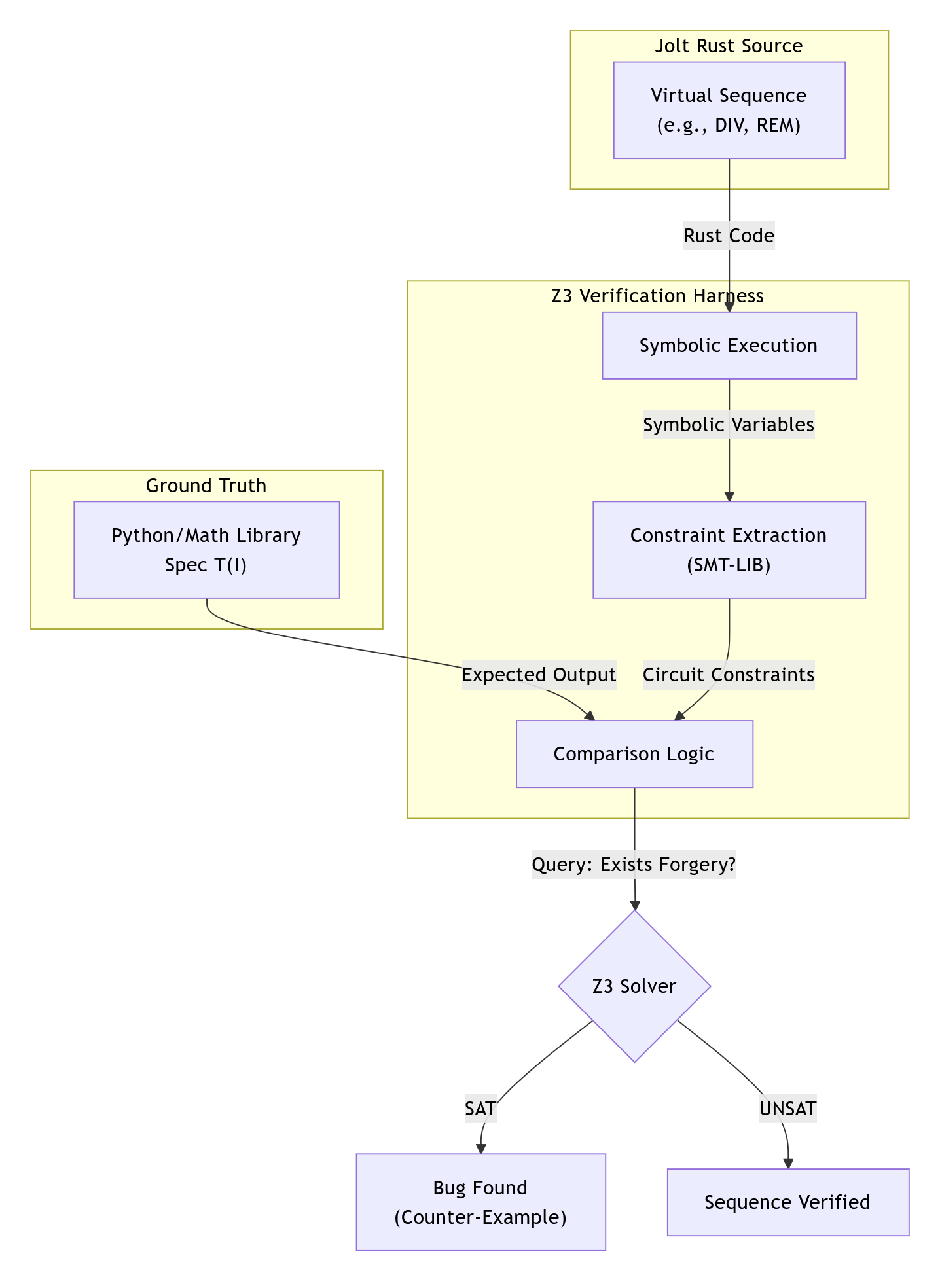
The Symbolic CPU
The core component is the SymbolicCpu struct. Unlike the standard emulator which operates on u64, this CPU operates on Z3 BitVectors (BV).
- Registers: Tracks as symbolic 64-bit values.
- Advice: Maintains a set of advice variables . When a
VirtualAdviceinstruction is executed, a new unconstrained symbolic variable is created and injected into the register file. - Asserts: Collects boolean constraints (e.g.,
VirtualAssertEQ) generated during execution.
Symbolic Execution
The symbolic_exec function acts as an interpreter, mapping Jolt Instruction variants to Z3 bit-vector operations BV
symbolic_exec(Instruction, State) -> NextState
Standard operations map directly (e.g., ADD -> bvadd), while virtual operations utilize Z3's logic for shifting and arithmetic.
Verification Macros
The test_sequence! macro generates two distinct tests for each instruction:
A. Correctness (test_correctness)
Proves that the Jolt sequence matches the RISC-V specification.
Property: Jolt(input) == RISC-V-Spec(input)
- Setup: Creates a
SymbolicCpu. - Spec Execution: Runs the "Ground Truth" closure on
cpu_expected. - Jolt Execution: Expands the instruction into its virtual sequence and symbolically executes it on the main
cpu. - Query:
Exists input s.t. (cpu.regs != cpu_expected.regs) AND (Asserts are satisfied)- UNSAT: The sequence is correct.
- SAT: A bug was found. The solver provides a counter-example.
B. Consistency (test_consistency)
Proves that the sequence is deterministic, even when relying on prover advice. We define the consistency query by duplicating the execution with independent advice variables A1 and A2.
Property: (Asserts(A1) AND Asserts(A2)) => Out(A1) == Out(A2)
- Setup: Creates two CPUs with identical initial registers (
x1 == x2). - Dual Execution: Executes the sequence on both.
VirtualAdvicegenerates distinct variables (a1for CPU 1,a2for CPU 2). - Query:
Exists input, A1, A2 s.t. (cpu1.regs != cpu2.regs) AND (Asserts1 AND Asserts2 are satisfied)- UNSAT: The constraints are strong enough to force a single unique result.
- SAT: The sequence is under-constrained, allowing multiple valid outputs.
2. R1CS Constraints (cpu_constraints.rs)
This module verifies the lowest-level circuits that enforce the CPU's state transitions, ensuring Consistency: for a given state and input , there exists exactly one valid next state .
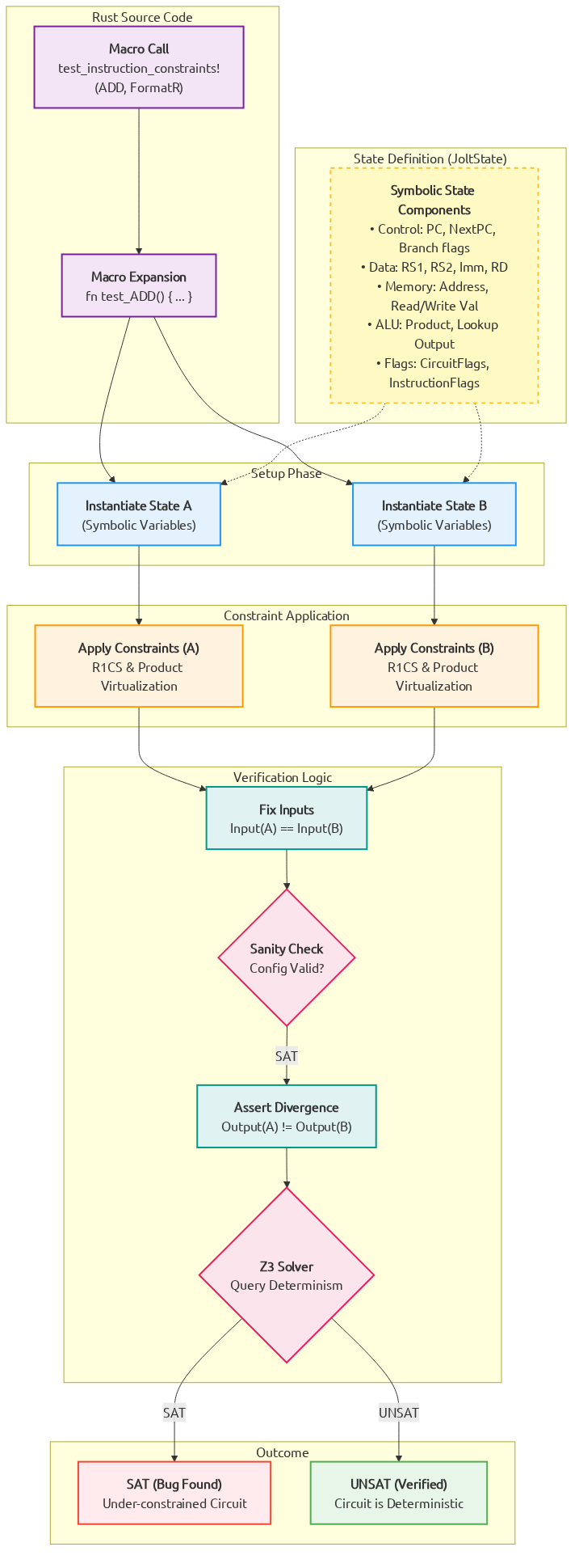
What defines a State?
In the R1CS verifier, a state (JoltState) is a complete symbolic snapshot of a single execution cycle. It is defined by the following variables (modeled as Z3 Integers):
- Control Flow:
pc(current),next_pc(next),unexpanded_pc, andnext_is_noop(padding indicator). - Data Flow:
rs1_value,rs2_value(read inputs),rd_write_value(write-back), andimm(instruction immediate). - Memory Context:
ram_addr(destination address),ram_read_value, andram_write_value. - ALU Witnesses:
left_input,right_input,product(multiplier output), andlookup_output. - System Signals:
CircuitFlags(e.g.,Add,Store,Jump) andInstructionFlags(e.g.,IsRdNotZero,Branch).
Consistency Check (do_test)
The verifier searches for non-deterministic transitions. We verify that the transition function is well-defined:
Property: C(S, I, S1) AND C(S, I, S2) => S1 == S2
- Dual States: Create symbolic states
S1andS2. - Constrain: Apply both R1CS and Product constraints to both states.
- Fix Inputs: Force both states to have identical inputs (same PC, flags, memory reads, and register values).
- Query:
Exists S, I, S1, S2 s.t. S1.outputs != S2.outputs- UNSAT: The circuit is sound (Deterministic).
- SAT: The circuit is under-constrained. The solver found a non-deterministic transition where the same input allows multiple valid next states.
NOTE: All the symbolic variables are modelled using integer arithmetic instead of finite field, which could cause slightly different behaviours. The harness only enforces consistency checks on the r1cs constraints, full formal verification is only guaranteed after correctness modelling against correct RISC-V spec.
Interpreting Results
When the test suite runs (cargo test -p z3-verifier -- --nocapture), it outputs SAT or UNSAT. A SAT result indicates a failure in verification.
Bit-Width Scaling (Virtual Sequences)
Some virtual sequences (notably those involving division/remainder or high-half multiplication) can be very slow at full 64-bit bitvector width. The virtual_sequences harness supports running the same checks at a scaled-down BitVec width to keep solver runtime manageable while preserving "boundary-condition" structure (e.g., 63 → n-1, 32 → n/2, all-ones masks, signed mins).
Set Z3_VERIFIER_BV_BITS to a power of two in [8, 64] (default: 64):
Z3_VERIFIER_BV_BITS=8 cargo test -p z3-verifier virtual_sequences -- --nocapture
1. Correctness Failures (Logic Bugs)
Symptom: test_..._correctness fails.
Meaning: The verifier found a concrete set of inputs where Jolt's output disagrees with the Spec.
Fix: Analyze the provided counter-example. If the logic in symbolic_exec is correct, the virtual sequence in jolt-prover-legacy is likely buggy.
2. Consistency Failures (Under-Constrained Advice)
Symptom: test_..._consistency fails.
Meaning: A malicious prover can choose different advice values to produce different final results, satisfying all constraints. Usually consistency failures in advice also lead to correctness failures since we can find an advice which leads to incorrect results.
Fix: The virtual sequence is missing validation. Add assertions (e.g., VirtualAssertEQ) to tightly constrain the advice.
3. R1CS Consistency Failures
Symptom: test_... in cpu_constraints fails.
Meaning: The R1CS constraints allow multiple next states for the same input.
Fix: Identify the unconstrained variable (e.g., rd_write_value). Add a constraint in crates/jolt-prover-legacy/src/zkvm/r1cs/constraints.rs to force this value to a deterministic state.
Appendix
This section includes supplementary background relevant to Jolt.
- Terminology and nomenclature
- Multilinear extensions
- Sumcheck
- Polynomial commitment schemes
- Memory checking and lookup arguments
- RISC-V
- Jolt 0.1.0
- Additional resources
Terminology and nomenclature
🚧 These docs are under construction 🚧
👷If you are urgently interested in this specific page, open a Github issue and we'll try to expedite it.👷
Multilinear Extensions
A function defined on the -dimensional boolean hypercube has a unique multilinear extension (MLE) : the unique polynomial of degree at most 1 in each variable that agrees with on all boolean inputs. Concretely,
The product term is the equality polynomial , which equals 1 when on the boolean hypercube and interpolates smoothly elsewhere.
MLEs are the central data structure in sumcheck-based proof systems: the sumcheck protocol operates over multilinear polynomials, and essentially all witness data in Jolt is represented as MLEs.
For a more formal introduction, see Section 3.5 of Proofs, Arguments, and Zero Knowledge.
Representation
An MLE over variables is stored as a vector of evaluations over the boolean hypercube . The -th entry of this vector stores where is the binary representation of . Jolt uses big-endian indexing: the most significant bit of corresponds to .
Variable binding
Given represented by evaluations, binding the most significant variable to a challenge produces a new MLE represented by evaluations. For each index :
where and for the same suffix . This is a single pass. Binding the least significant variable instead pairs even/odd entries: .
Which variable gets bound in each round is determined by the BindingOrder: HighToLow (most significant first) or LowToHigh (least significant first).
Implementations in Jolt
The MLE implementations live in crates/jolt-prover-legacy/src/poly/. All are unified under the MultilinearPolynomial<F> enum (multilinear_polynomial.rs), which dispatches binding and evaluation to the appropriate concrete type. The two most common representations are DensePolynomial and CompactPolynomial.
DensePolynomial
DensePolynomial<F> (dense_mlpoly.rs) is the straightforward representation: a Vec<F> of field elements. This is the baseline MLE type used when coefficients are full-sized field elements.
Binding operates in-place on the evaluation vector. In HighToLow order, the vector is split into left and right halves (corresponding to the most significant variable being 0 or 1) and interpolated:
#![allow(unused)]
fn main() {
let (left, right) = self.Z.split_at_mut(n);
left.iter_mut().zip(right.iter()).for_each(|(a, b)| {
    *a += r * (*b - *a);
});
}
In LowToHigh order, adjacent even/odd pairs are interpolated instead:
#![allow(unused)]
fn main() {
for i in 0..n {
    self.Z[i] = self.Z[2 * i] + r * (self.Z[2 * i + 1] - self.Z[2 * i]);
}
}
Both orders have parallel variants (bind_parallel) that use Rayon. The HighToLow parallel path binds in place, while the LowToHigh parallel path cannot.
CompactPolynomial
CompactPolynomial<T, F> (compact_polynomial.rs) stores coefficients as small scalars of type T (implementing the SmallScalar trait: bool, u8, u16, u32, u64, u128, i64, i128) rather than full field elements. This is the "pay-per-bit" representation that makes Dory commitments efficient.
The polynomial maintains two storage vectors:
coeffs: Vec<T>— the original small-scalar coefficients (immutable after construction).bound_coeffs: Vec<F>— field elements materialized lazily on the first bind.
Binding has two phases. On the first bind, coefficients are promoted from small scalars to field elements using SmallScalar arithmetic that avoids overflow:
#![allow(unused)]
fn main() {
// For a pair (a, b) of small scalars:
match a.cmp(&b) {
    Ordering::Equal => a.to_field(),
    Ordering::Less  => a.to_field() + r * (b - a).to_field(),
    Ordering::Greater => a.to_field() - r * (a - b).to_field(),
}
}
After this first bind populates bound_coeffs, subsequent binds operate on field elements identically to DensePolynomial.
The MultilinearPolynomial enum has a variant for each scalar type (U8Scalars, U16Scalars, I128Scalars, etc.), so dispatch is monomorphized and the small-scalar optimizations apply throughout the sumcheck hot loop.
Other specialized representations
Several other MLE types in crates/jolt-prover-legacy/src/poly/ exploit structure specific to Jolt's witness polynomials:
OneHotPolynomial(one_hot_polynomial.rs): Stores only the index of the single nonzero entry per cycle rather than a dense vector of 0s and 1s. Used for and polynomials in Twist and Shout.RaPolynomial(ra_poly.rs): A state machine that lazily materializes the (or ) polynomial across sumcheck rounds (Round1 Round2 Round3 RoundN), keeping memory proportional to the address-space size rather than until the final rounds.RLCPolynomial(rlc_polynomial.rs): Represents a random linear combination of multiple polynomials. Dense components are eagerly combined; one-hot components are stored as(coefficient, polynomial)pairs and combined lazily during evaluation. Arises in the PCS opening proof.EqPolynomial(eq_poly.rs): The equality MLE , commonly used as a building block in sumcheck and MLE evaluation.
The Sumcheck Protocol
Adapted from the Thaler13 exposition. For a detailed introduction to sumcheck see Chapter 4.1 of the textbook.
Suppose we are given a -variate polynomial defined over a finite field . The purpose of the sumcheck protocol is to compute the sum:
In order to execute the protocol, the verifier needs to be able to evaluate for a randomly chosen vector . Hence, from the verifier's perspective, the sumcheck protocol reduces the task of summing 's evaluations over inputs (namely, all inputs in ) to the task of evaluating at a single input in .
The protocol proceeds in rounds as follows. In the first round, the prover sends a polynomial , and claims that
Observe that if is as claimed, then . Also observe that the polynomial has degree , the degree of variable in . Hence can be specified with field elements. In our implementation, will specify by sending the evaluation of at each point in the set . (Actually, the prover does not need to send , since the verifier can infer that , as if this were not the case, the verifier would reject).
Then, in round , chooses a value uniformly at random from and sends to . We will often refer to this step by saying that variable gets bound to value . In return, the prover sends a polynomial , and claims that
The verifier compares the two most recent polynomials by checking that , and rejecting otherwise. The verifier also rejects if the degree of is too high: each should have degree , the degree of variable in .
In the final round, the prover has sent which is claimed to be . now checks that (recall that we assumed can evaluate at this point). If this test succeeds, and so do all previous tests, then the verifier accepts, and is convinced that .
Polynomial Commitment Schemes
Polynomial commitment schemes (PCS) are a core cryptographic primitive in proof systems, including zkVMs. At a high level, they allow a prover to commit to a polynomial and later open that commitment (i.e. evaluate the underlying polynomial) at a point chosen by the verifier, while ensuring the binding property (the prover cannot change the polynomial after committing to it).
This mechanism is powerful because it allows succinct verification of polynomial relationships without the prover needing to reveal the entire polynomial. The verifier only learns the evaluation at chosen points.
Usage
A PCS comprises three algorithms (plus sometimes a preprocessing step): , , and . In the context of a larger proof system like Jolt, polynomial commitment schemes are typically used in some variation of the following flow:
- Depending on the PCS, there may be a preprocessing step, where some public data is generated. This data may be needed for , , or . This preprocessing could involve a trusted setup (if not, it is called a transparent setup/PCS).
- Prover commits to polynomial , and the commitment is sent to the verifier.
- In some subsequent part of the proof system, the prover and verifier arrive at some claimed evaluation (typically for a random point ). For example, this claimed evaluation might be an output claim of a sumcheck.
- The prover provides an opening proof for the evaluation, and sends the proof to the verifier.
- The verifier then verifies the opening proof. If the verification succeeds, then the verifier can rest assured that as claimed.
Role in Jolt
In Jolt, the prover commits to several witness polynomials derived from the execution trace being proven. These polynomial commitments are used extensively to tie together the various algebraic claims generated during proving. Jolt currently uses Dory as its polynomial commitment scheme. Dory provides an efficient method for committing to and opening one-hot polynomials, while supporting batch openings across many claims with relatively low overhead.
Further Reading
For a more formal and detailed introduction to polynomial commitment schemes, we recommend Section 7.3 of Justin Thaler’s Proofs, Arguments, and Zero Knowledge. That section explains how polynomial commitments integrate with interactive proof protocols such as GKR, and why they are essential for constructing succinct arguments.
Memory checking and lookup arguments
🚧 These docs are under construction 🚧
👷If you are urgently interested in this specific page, open a Github issue and we'll try to expedite it.👷
RISC-V
RISC-V is an open-source instruction set architecture (ISA) based on reduced instruction set computer (RISC) principles. Every RISC-V implementation includes a base integer ISA, with optional extensions for additional functionality.
Supported Instructions
Jolt currently supports the RV64IMAC instruction set, comprising the 64-bit integer instruction set (RV64I), the integer multiplication/division extension (RV64M), the atomic memory operations extension (RV64A), and the compressed instruction extension (RV64C).
RV64I (base)
RV64I is the base 64-bit integer instruction set: 32 registers (x0--x31, each 64 bits wide, with x0 hardwired to zero), 32-bit fixed-width instructions, and a load/store architecture (all arithmetic operates on registers; memory is accessed only via dedicated load/store instructions with base-plus-offset addressing). It provides arithmetic, logical, shift, branch, and jump operations.
For detailed instruction formats and encoding, refer to chapter 2 of the specification.
"M" extension (integer multiply/divide)
Adds signed and unsigned multiplication (MUL, MULH, MULHU, MULHSU) and division/remainder (DIV, DIVU, REM, REMU), plus their 32-bit W-type variants. Divide-by-zero produces a well-defined result rather than a trap.
For detailed instruction formats and encoding, refer to chapter 7 of the specification.
"A" extension (atomics)
Adds atomic read-modify-write operations (AMOSWAP, AMOADD, AMOAND, AMOOR, AMOXOR, AMOMIN, AMOMAX) and load-reserved/store-conditional (LR/SC) pairs, each in word (32-bit) and doubleword (64-bit) variants.
Jolt's LR/SC implementation
Jolt implements LR/SC using virtual sequences with a pair of width-specific reservation registers:
reservation_w(virtual register 32) -- used byLR.W/SC.Wfor word (32-bit) reservationsreservation_d(virtual register 33) -- used byLR.D/SC.Dfor doubleword (64-bit) reservations
The two reservation registers enforce width-matched pairing: LR.W sets reservation_w and clears reservation_d; LR.D does the reverse. This cross-clear means SC.W after LR.D (or SC.D after LR.W) will always fail, since the SC checks only its own width's reservation register.
The SC failure path uses prover-supplied VirtualAdvice constrained to . On success, a constraint forces the reservation address to match rs1, and rs2 is stored to memory. On failure, the store is a no-op (the original memory value is written back). The destination register rd receives 0 on success, 1 on failure. Both reservation registers are always cleared at the end of any SC instruction, per the RISC-V specification.
For the constraint design and soundness argument, see RISC-V emulation. For the virtual register layout, see Registers.
For detailed instruction formats and encoding, refer to chapter 8 of the specification.
"C" extension (compressed instructions)
Provides 16-bit encodings for common operations, reducing binary size by ~25--30%. Compressed instructions map directly to their 32-bit RV64I equivalents and can be freely intermixed with them; the Jolt tracer expands them before execution.
For detailed instruction formats and encoding, refer to chapter 16 of the specification.
Compilation via LLVM
Jolt proves execution of RISC-V ELF binaries, which can be produced from any language with an LLVM frontend (Rust, C, C++, etc.). The jolt-sdk crate handles cross-compilation to the RISC-V target automatically via the #[jolt::provable] macro. The compilation pipeline is:
Source (Rust/C/C++) → LLVM IR → RISC-V ELF → Jolt tracer → proof
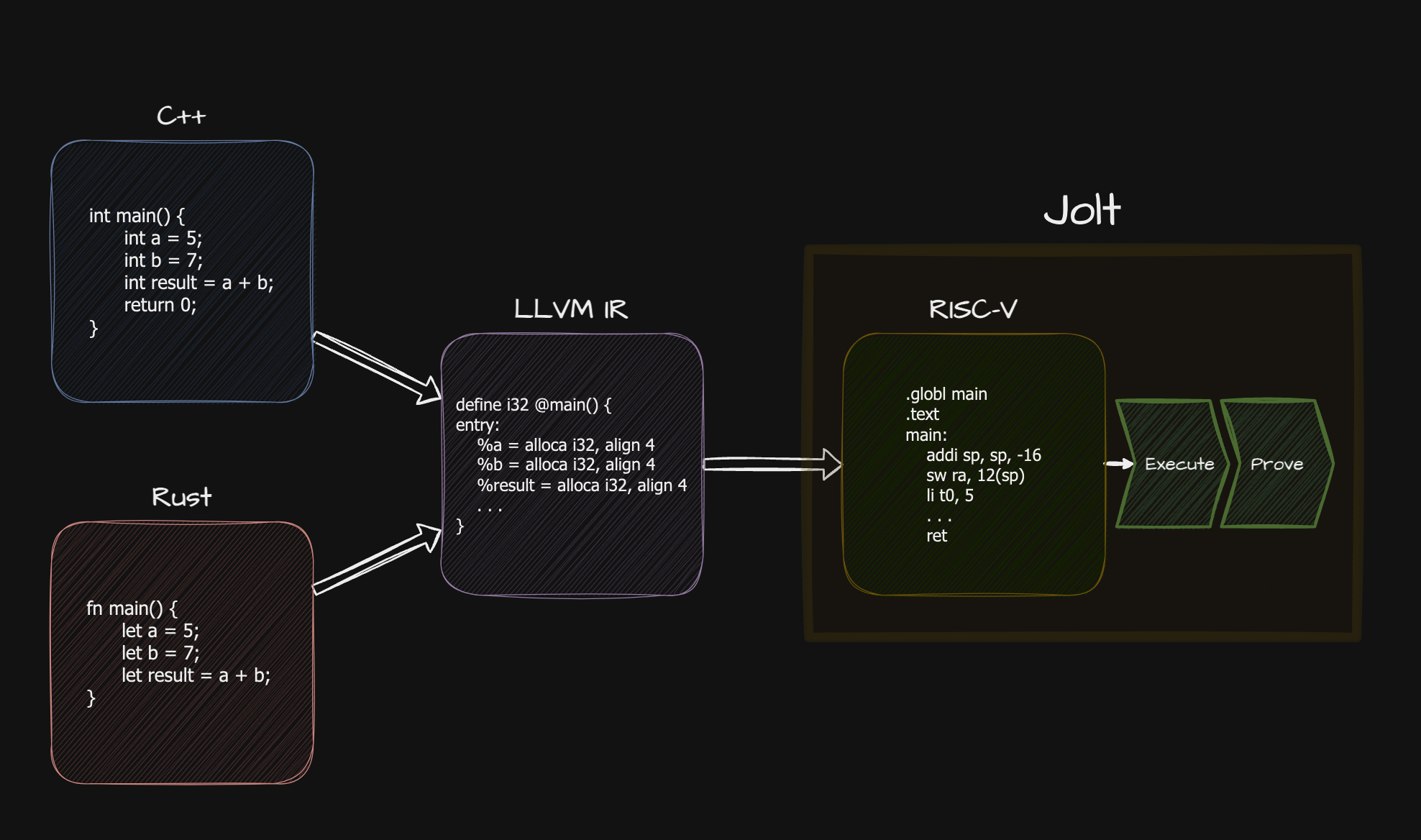
References
- RISC-V Specifications
- RV64I Base ISA Specification
- RISC-V Assembly Programmer's Manual
- LLVM RISC-V Backend Documentation
Jolt 0.1.0
🚧 These docs are under construction 🚧
👷If you are urgently interested in this specific page, open a Github issue and we'll try to expedite it.👷
Additional resources
🚧 These docs are under construction 🚧
👷If you are urgently interested in this specific page, open a Github issue and we'll try to expedite it.👷
Roadmap
This section describes the major features and improvements planned for Jolt. In rough order of proximity:
Streaming
Other zkVMs, when applied ``monolithically'' (meaning in non-recursive fashion), have prover memory requirements that grow linearly with the number of CPU cycles being proven. This translates to many GBs of space per million cycles proved.
The way other zkVMs address this issue is a technique commonly referred to as continuations. One breaks the CPU execution into ``shards'' (often consisting of about a million cycles each), prove each shard (more or less) independently, and then recursively aggregates the proofs. This leads to many complications and performance overheads.
Jolt is amenable to a different approach that we call the streaming prover. For arbitrarily long CPU executions, the Jolt prover can keep its memory usage bounded to a few GBs (plus the space required to simply run the program itself) without SNARK recursion. The time overhead of the streaming Jolt prover relative to the linear-space Jolt prover will be minimal, certainly well below a factor of 2x.
At a high level, the streaming Jolt prover works as follows. In each round of any invocation of the sum-check protocol within Jolt, each step of the CPU execution contributes independently to the prover's message in that round of sum-check. Hence, the prover can compute the required message in that round incrementally in small space as it runs the CPU from start to finish. This observation is very old (see [CTY11] and [Clover 2014] ).
The above sketch suggests that the streaming Jolt prover would have to perform a linear (in the cycle count) number of field operations per sum-check round. This is not at all the case in Jolt, for myriad reasons, some of which are sketched below (see [NTZ25] for details).
First, Twist and Shout are naturally streaming, in the sense that while they require up to rounds of sum-check where is the cycle count (here, 128 arises when primitive instructions take 128 bits of input), the first 128 rounds can be completed by the prover with just a few passes in total over the execution trace and a low-order amount of prover work.
Second, various optimizations to the Spartan-in-Jolt prover time are \emph{also} directly compatible with a streaming prover in the sense above: stream-ifying this prover algorithm does not actually lead to a significant slowdown compared to the linear-space version.
Third, recent improvements to streaming sum-check proving ensure that each pass the prover makes over the execution trace actually suffices to get the prover through many rounds rather than a single round (see [BCFFMMZ25] ).
Fourth, while the first "run" of the CPU is typically down serially, subsequent runs performed by the prover can be done in parallel.
Today, the Jolt prover is not streaming, using under 2 GB of memory per million cycles proved. Work to "stream-ify" the prover is underway. For all of the reasons above (and others) we expect the streaming prover to be almost as fast as the current linear-space implementation.
Recursion
🚧 These docs are under construction 🚧
👷If you are urgently interested in this specific page, open a Github issue and we'll try to expedite it.👷
On-chain verification
🚧 These docs are under construction 🚧
👷If you are urgently interested in this specific page, open a Github issue and we'll try to expedite it.👷